Partitions & Parallelism

Part II — The Data Abstractions · Module 3 of 18 Prerequisites: What is Spark?, Spark Architecture You will learn: what a partition really is, why it is the atomic unit of parallelism, how Spark decides how big partitions should be, what data locality buys you, how shuffles create a whole new set of partitions, and how to recognize and avoid the infamous small file problem.

---

The idea in one line

A partition is a chunk of your data that lives on one machine, and Spark processes one partition per task per core.

Everything in this module flows from that single sentence. In Module 02 we said "parallelism is capped by partition count." Now we earn that claim by looking at partitions up close.

---

What a partition actually is

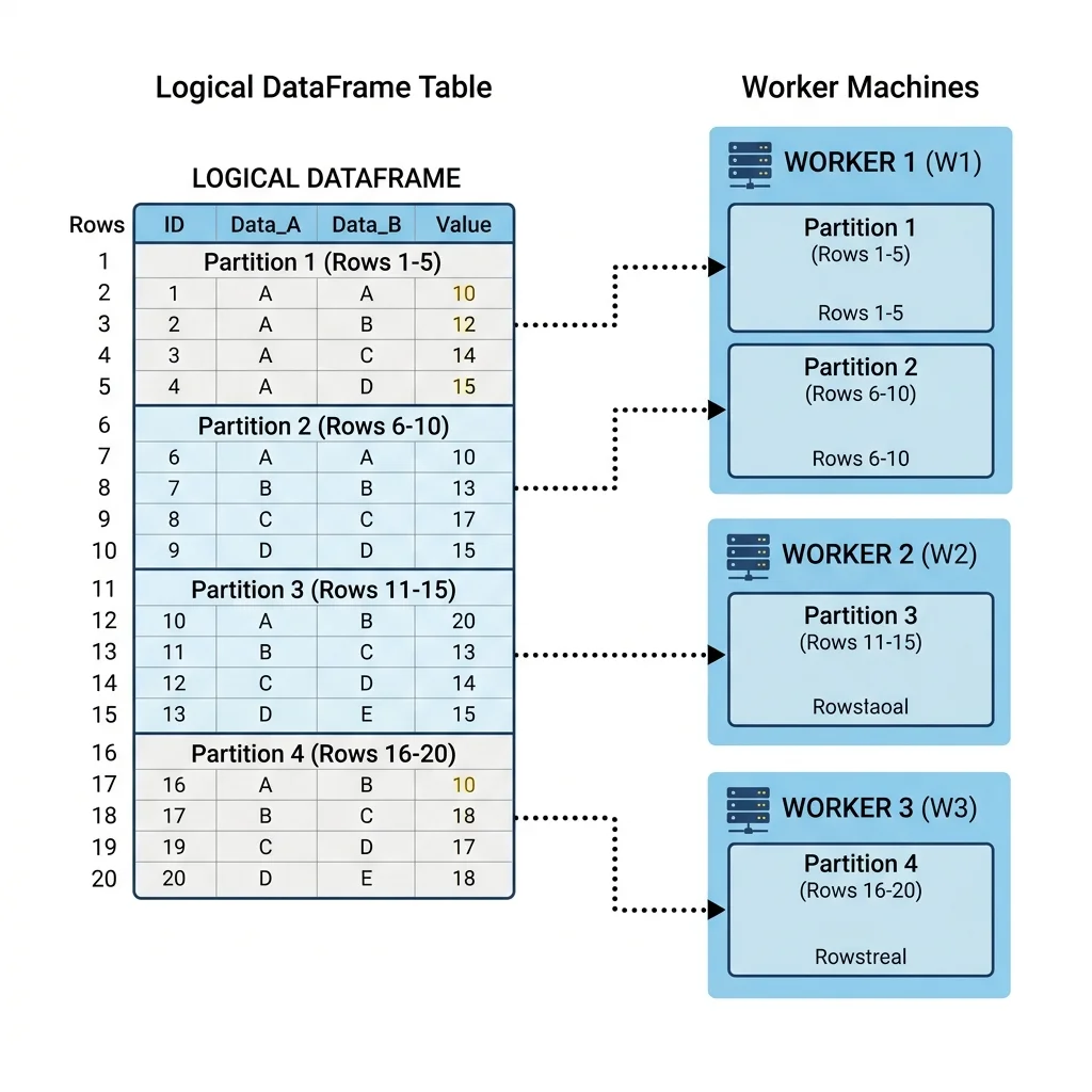
Your data is far too big for one machine — that was the whole reason for Spark. So Spark breaks the dataset into pieces called partitions. A partition is a physical collection of rows that resides on one physical machine in the cluster.

A DataFrame, then, is not one monolithic table sitting in one place. It is a logical table whose rows are physically scattered across the cluster as partitions. When you write df.filter(...), you're describing an operation on the whole logical table; Spark carries it out by running that filter independently on each physical partition, wherever it happens to live.

Analogy — a book split among readers. Imagine a 1,000-page book you need to proofread tonight. Alone, it's hopeless. So you tear it into ten 100-page sections (partitions) and hand one to each of ten friends (cores). Each friend proofreads their section independently and in parallel. The book is still "one book" conceptually, but physically it's ten stacks being worked on at once. That's a partitioned DataFrame.

There's an important layering here worth making explicit. Down at the storage level, your data already sits as physical blocks in a file system (HDFS, S3, Azure Blob). Spark maps those physical blocks into logical partitions in memory, represented to you as a DataFrame. You think in DataFrames; Spark thinks in partitions; the storage layer thinks in blocks.

---

Why partitions ARE parallelism

Here is the rule from Module 02, stated precisely: a partition is the atomic unit of parallelism. A single thread on a single CPU core processes exactly one partition at a time.

Because of that one-to-one binding, the number of partitions directly bounds how parallel your job can be. Two thought experiments make this vivid:

• Many executors, one partition. Suppose you have thousands of executor cores but your DataFrame has exactly one partition. Spark's active parallelism is... one. Only one core can touch that single partition; every other core sits idle. Enormous cluster, single-file execution.
• Many partitions, one executor. Now flip it: hundreds of partitions but only a single executor core. Parallelism is again one, because there's only one worker to process them — it just chews through the partitions one after another.

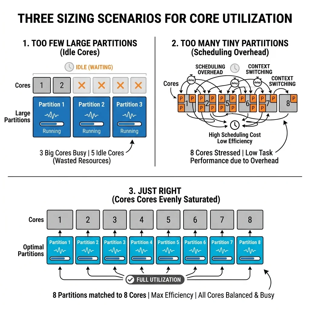
Real parallelism requires both enough partitions and enough cores, matched to each other. This is why partition count is one of the first things an experienced engineer checks when a job is mysteriously slow: the cluster might be huge, but if the data is in three partitions, only three cores are ever working.

The balance you're aiming for: keep a partition-to-core ratio of at least 1:1, and often 2:1 or 3:1 is better. A slight surplus of partitions keeps every core busy — when one core finishes its partition, there's another waiting, so no core goes idle waiting for the slowest one. We'll quantify this in the tuning module.

---

Data locality: move the computation, not the data

Recall from Module 01 that Spark prefers to process data where it already lives. Partitions are where that principle becomes concrete.

Moving data across a network is slow and expensive compared to reading it from a local disk or memory. So Spark tries to schedule each task on the executor that is physically closest to the partition it needs — ideally the very machine already holding that block of data. This is called data locality, and it minimizes network traffic by shipping the (tiny) computation to the (large) data rather than the reverse.

Analogy — library branches. You need facts from books held at ten different library branches across a city. You could truck every book to one central desk and read them there (moving the data — slow, congested roads). Or you could send one researcher to each branch to read on-site and phone in a one-line summary (moving the computation — fast). Data locality is Spark choosing the second strategy by default.

You rarely configure locality directly, but understanding it explains a lot of Spark's behavior — including why the shuffle we're about to meet is so costly: a shuffle deliberately breaks locality by forcing data to move across the network.

---

Sizing partitions: the Goldilocks problem

If partitions drive parallelism, how big should each one be? This is a "not too big, not too small" balancing act.

• Too few / too big: not enough partitions to keep all your cores busy, and individual partitions may be too large to fit comfortably in an executor's memory, causing spills to disk.
• Too many / too small: massive scheduling overhead (Spark launches a task per partition) and the small file problem (below). Each tiny task has fixed overhead that dwarfs its actual work.

Spark gives you a knob for the input side. When reading files, the size of each logical partition is governed by:

# Default is 128 MB. This controls the target size of each partition when READING files.
spark.conf.set("spark.sql.files.maxPartitionBytes", 128 * 1024 * 1024)  # 128 MB

For reference, on-disk file blocks are commonly 64 MB to 128 MB, and Spark's default spark.sql.files.maxPartitionBytes is 128 MB — deliberately in the same ballpark, so one partition roughly corresponds to one block. That default is sensible for a lot of workloads; you tune it when your partitions come out too big or too small for your cluster.

Inspecting and changing partition count

You can always check and adjust how many partitions a DataFrame has:

# How many partitions does this DataFrame currently have?
print(df.rdd.getNumPartitions())

# Increase partitions (this triggers a full shuffle — see Module 07). Use to grow parallelism.
more = df.repartition(200)

# Decrease partitions WITHOUT a full shuffle — merges adjacent partitions on the same node.
fewer = df.coalesce(10)

Two operations, one crucial difference we'll revisit in Module 17: repartition() reshuffles all the data across the network (expensive, but can both increase and evenly rebalance partitions), while coalesce() just merges neighboring partitions locally (cheap, but only reduces the count). Rule of thumb: coalesce to shrink, repartition to grow or to fix imbalance.

---

Shuffle partitions: a different animal

So far we've discussed input partitions — how Spark chunks data when it reads it. But there's a second, separate population of partitions created during execution, and confusing the two is a classic beginner trap.

When you run a wide transformation — something like groupBy(), join(), or orderBy() that requires data to move across the cluster — Spark performs a shuffle (the whole of Module 07). The shuffle produces a fresh set of partitions called shuffle partitions, and these are controlled by a completely different setting:

# Governs the number of partitions AFTER a shuffle (groupBy, join, orderBy...). Default: 200.
spark.conf.set("spark.sql.shuffle.partitions", 200)

The default is 200, and that default is one of the most common causes of poor performance for beginners. Here's why: 200 is far too many for a small or local dataset. If you're processing a few megabytes, Spark still dutifully creates 200 shuffle partitions — 200 tiny tasks, each with scheduling and network overhead, most containing almost no data. For local development or small/streaming workloads, dial this down to match your executor cores (e.g., 5, 8, or 16). For genuinely large workloads, you may need to raise it to keep partitions from growing too big and spilling to disk.

Two knobs, don't mix them up:

• spark.sql.files.maxPartitionBytes → sizes partitions when reading files (default 128 MB).
• spark.sql.shuffle.partitions → counts partitions after a shuffle (default 200).

A huge fraction of "why is my tiny job so slow?" questions trace back to the shuffle default of 200.

---

The small file problem

The flip side of "too many tiny partitions" shows up both when reading and when writing: the small file problem.

If your data is stored as thousands of tiny files, or your job writes thousands of tiny output files, you pay a steep, often invisible tax:

• The file system (e.g., HDFS) must track metadata for every single file — and metadata operations don't come free.
• Spark's scheduler must launch a separate task to read every single file, so you drown in per-task overhead — directory listing, task setup, teardown — with barely any real computation in between.

The fix on the write side is to control output file size directly:

# Cap records per output file so you write fewer, healthier-sized files
# instead of thousands of tiny ones.
df.write.option("maxRecordsPerFile", 50000).parquet("/tmp/output")

The guiding target: aim for output files of at least a few tens of megabytes rather than a swarm of kilobyte-sized ones. When reading a directory that's already full of small files, coalesce() after the read (or upstream compaction) helps consolidate them. Either way, the instinct to cultivate is: fewer, fatter files and partitions beat many tiny ones.

Analogy — shipping a warehouse. Shipping 10,000 items is far cheaper in a few well-packed pallets than in 10,000 individually addressed envelopes. Each envelope needs its own label, postage, and handling (per-task overhead); the pallets amortize all that. Small files are the envelopes; healthy partitions are the pallets.

---

Key takeaways

• A partition is a chunk of a DataFrame's rows living on one machine; a DataFrame is a logical table physically scattered as partitions over storage blocks.
• A partition is the atomic unit of parallelism — one core runs one task on one partition at a time — so partition count bounds parallelism. You need enough partitions and enough cores, matched (aim for a 2:1–3:1 partition-to-core ratio).
• Data locality means Spark ships the computation to the data to avoid slow network transfer; shuffles are costly precisely because they break locality.
• Partition sizing is a Goldilocks problem: too big underuses cores and risks memory spills; too small drowns you in scheduling overhead.
• Two separate knobs, often confused: spark.sql.files.maxPartitionBytes (read-time, default 128 MB) and spark.sql.shuffle.partitions (post-shuffle count, default 200 — usually too high for small jobs).
• Use coalesce() to shrink partitions cheaply and repartition() to grow or rebalance them (at the cost of a shuffle).
• The small file problem — thousands of tiny files/partitions — bloats metadata and per-task overhead; prefer fewer, fatter files (e.g., via maxRecordsPerFile).

---

Check your understanding

1. You run a job on a 100-core cluster, but a DataFrame has only 4 partitions. What is the maximum number of cores that can do useful work, and why?
2. What's the difference between spark.sql.files.maxPartitionBytes and spark.sql.shuffle.partitions? Which one is the usual culprit when a small job runs surprisingly slowly?
3. You need to reduce a DataFrame from 500 partitions to 50 before writing it out. Would you reach for coalesce() or repartition(), and what's the trade-off?

---

Up next

RDDs, DataFrames, Datasets — RDDs vs. DataFrames vs. Datasets. We've been saying "DataFrame" throughout — but it's one of three core data abstractions in Spark. Next we compare all three, explain why DataFrames are usually the right default, and show what you gain (and give up) with each.