The Shuffle

Part III — The Execution Engine · Module 7 of 18 Prerequisites: Transformations & Actions (narrow vs. wide), Partitions & Parallelism, Lazy Evaluation & the DAG You will learn: what a shuffle actually is, why certain operations force one, the four phases it moves through, exactly why it's the most expensive thing Spark does, how it creates stage boundaries, and the practical toolkit for reducing shuffles.

---

The most expensive operation in Spark

We've been building toward this module for a while. Every time you saw the words "wide transformation," "Exchange," or "the most expensive operation," we were pointing here. So let's state it directly:

A shuffle is the process of redistributing data across partitions and executors so that related records end up together. It happens whenever an operation needs data that is currently scattered across many partitions to be regrouped — typically by key.

The shuffle is unavoidable for certain operations (you genuinely cannot group by a key without bringing all rows with that key together), but it is also the number-one performance concern in Spark. If you master one performance concept from this entire guide, make it this one: know where your shuffles are, and move as little data through them as possible.

Analogy — reorganizing a conference by track. Picture a conference where 500 attendees are seated randomly across ten rooms. You now announce: "Everyone regroup so that all the AI people are in Room 1, all the Security people in Room 2, all the Data people in Room 3." Chaos erupts — hundreds of people stand up, stream through the hallways, and re-sort themselves into new rooms. That mass migration through the corridors is a shuffle. The hallways are your network; the crowd is your data; and the whole thing is slow precisely because everyone has to move at once.

---

Why a shuffle happens

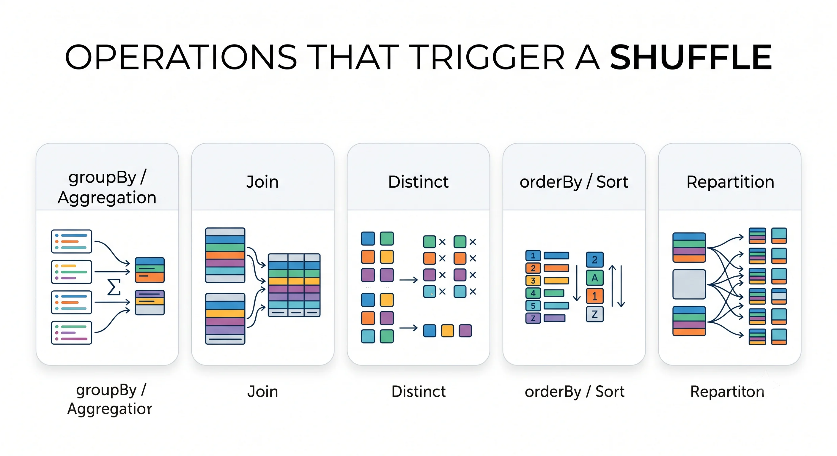
A shuffle is triggered by wide transformations (Module 05) — operations where computing one output partition requires input from many partitions. The infographic that seeds this guide lists the usual causes, and they all share one trait: they need all records sharing a key to be in the same place.

• Grouping — groupBy() / agg(): to sum sales per city, every row for a given city must land together.
• Joining — join(): to match rows across two tables on a key, matching keys must be colocated.
• Distinct — distinct() / dropDuplicates(): to detect duplicates, identical rows must meet.
• Sorting — orderBy() / sort(): a global order requires cross-partition reordering.
• Explicit repartitioning — repartition(), reduceByKey(): you're literally asking Spark to redistribute.

The common thread is worth stating as a rule you can apply on sight: any operation that reasons across keys — grouping, joining, deduping, globally sorting — needs a shuffle. Operations that reason within a single row (filter, select, withColumn) never do. When you scan a query for cost, this is the filter you run in your head.

---

Inside a shuffle: the four phases

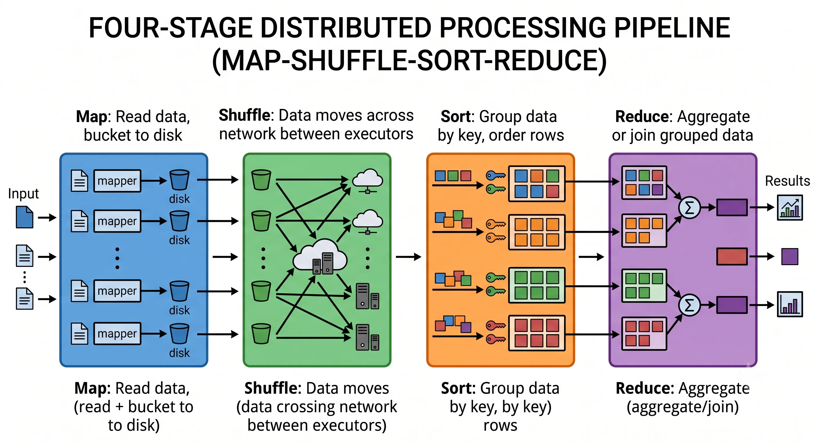
A shuffle isn't a single instantaneous event — it moves through phases. Following the framing from the "9 Concepts" infographic, we can break it into four:

1. Map phase — Each task reads its input partition and computes, for every record, which output partition it belongs to (based on the key's hash). It writes the records out, bucketed by destination, into shuffle files on local disk. This is the "prepare to move" step.
2. Shuffle phase — The data is redistributed across the network. Each destination executor fetches the buckets meant for it from every other executor. This is the mass migration — the corridor crush from our analogy — and the part that saturates the network.
3. Sort phase — On the receiving side, data is organized (often sorted by key) so that all records for a given key are grouped and ready.
4. Reduce phase — The actual aggregation or join happens on the now-colocated data — sums are computed, matching rows are joined — and results are produced.

The order to remember is map → shuffle → sort → reduce: prepare locally, move across the network, organize on arrival, then compute.

---

Why it's so expensive: network AND disk

Narrow transformations stay local and can be pipelined in memory. A shuffle is the opposite on every axis, and it pays two separate I/O taxes:

• Network I/O — Data physically crosses the network from every source executor to every destination executor. Network transfer is orders of magnitude slower than reading from local memory, and it breaks the data locality that Module 03 worked so hard to preserve.
• Disk I/O — For fault tolerance, Spark writes the intermediate shuffle files to local disk during the map phase before the exchange. If a downstream task fails, Spark can re-fetch these files instead of recomputing everything. That safety costs disk writes and reads on top of the network cost.

So a wide transformation involves computation + disk writes + network transfer + disk reads + more computation — versus a narrow transformation's single in-memory pass. That's the entire reason "shuffle = expensive" is drilled so hard. It's not one costly thing; it's a stack of costly things.

Shuffles create stage boundaries

There's a structural consequence too, connecting back to Module 02's vocabulary. A shuffle is exactly where Spark splits a job into stages. Everything Spark can pipeline without moving data becomes one stage; the moment a shuffle is required, the current stage ends and a new one begins after the exchange. This is why, when you read a query plan or the Spark UI, stage boundaries and Exchange nodes line up with your shuffles. Counting stages is another way of counting shuffles.

Shuffle partitions, revisited

Recall the second partition knob from Module 03: spark.sql.shuffle.partitions, default 200. This is the setting that controls how many partitions the shuffle produces on the output side. Its default is a frequent performance trap:

# For small or local datasets, 200 shuffle partitions creates 200 tiny tasks — mostly overhead.
# Match it roughly to your available executor cores instead.
spark.conf.set("spark.sql.shuffle.partitions", 8)

Too high, and every shuffle spawns hundreds of near-empty tasks drowning in scheduling overhead. Too low on a big dataset, and each shuffle partition grows large enough to spill to disk. Tuning this per-workload is one of the highest-leverage adjustments you can make — we return to it in Module 17.

---

Reducing shuffles: the practical toolkit

You cannot eliminate shuffles entirely — some regrouping is genuinely required by your logic. But you can dramatically cut how much they cost. Here is the working engineer's checklist, each item with the intuition behind it.

1. Filter early — shrink the data before it moves

The cheapest byte to shuffle is the one you never shuffle. Apply filter()/where() before a wide transformation so less data enters the shuffle. (And thanks to lazy evaluation and predicate pushdown from Module 06, Spark often does this reordering for you — but writing it clearly helps.)

# Good: filter first, THEN group — far less data crosses the network.
result = (df
          .filter(col("country") == "Japan")   # narrow, shrinks data first
          .groupBy("city")                       # wide, but on much less data
          .sum("amount"))

2. Use broadcast joins for small tables

When you join a huge table with a small lookup table, you don't have to shuffle both. Spark can broadcast the small table — send a full copy to every executor — so the join happens locally with no shuffle of the big table at all. This is important enough to get its own treatment in Module 16; for now, know it's the single biggest shuffle-killer for joins.

from pyspark.sql.functions import broadcast

# Broadcast the small dimension table to avoid shuffling the large fact table.
joined = large_fact_df.join(broadcast(small_dim_df), "id")

3. Partition and bucket your stored data wisely

If data is physically partitioned on disk by a column you often filter on (e.g., date), Spark skips whole directories — less data read, less shuffled. If two large tables are bucketed on their join key at write time, Spark can join them without a shuffle because matching keys are already colocated. (Both covered in Modules 16–17.)

4. Prefer aggregating at the right stage, and avoid needless wide ops

Don't call distinct() or orderBy() "just in case" — each is a full shuffle. Aggregate as early as possible so the data flowing into later stages is already smaller. Every wide operation you can drop or defer is a shuffle you don't pay for.

5. Cache before a repeated shuffle-heavy computation

If a shuffled result is reused across multiple actions, cache it so the expensive shuffle runs once, not once per action (Module 15).

The mental model: you can't avoid the corridor crush entirely, but you can (1) send fewer people through it, (2) let small groups teleport (broadcast) instead of walking, and (3) pre-seat people so some regrouping isn't needed at all. Every shuffle optimization is a version of one of those three moves.

---

Key takeaways

• A shuffle redistributes data across partitions/executors so records sharing a key end up together. It's triggered by wide transformations — groupBy, join, distinct, orderBy, repartition.
• The rule of thumb: operations that reason across keys need a shuffle; operations that reason within a row don't.
• A shuffle proceeds in four phases — map → shuffle → sort → reduce: bucket to local disk, move across the network, organize by key on arrival, then aggregate/join.
• It's expensive because it pays both network I/O and disk I/O (intermediate shuffle files are written to disk for fault tolerance), unlike a narrow transformation's single in-memory pass.
• Each shuffle is a stage boundary; Exchange nodes in a plan = shuffles. spark.sql.shuffle.partitions (default 200) controls output partition count and is a common tuning target.
• Reduce shuffles by: filtering early, using broadcast joins for small tables, partitioning/bucketing stored data, avoiding needless wide ops, and caching reused shuffled results.

---

Check your understanding

1. Why does groupBy("city") require a shuffle but withColumn("tax", col("amount") * 0.1) does not? Frame your answer in terms of "reasoning across keys" vs. "within a row."
2. Name the two kinds of I/O a shuffle incurs and explain why the disk one exists even though the data is "just moving across the network."
3. You join a 2 TB fact table with a 5 MB lookup table and it's painfully slow. What one technique would you try first, and why does it avoid shuffling the big table?

---

Up next

Catalyst & Tungsten — Catalyst & Tungsten. We've repeatedly credited "the optimizer" for rewriting queries and "Tungsten" for fast binary storage. Next we open both black boxes: Catalyst's four optimization phases and Tungsten's whole-stage code generation — the machinery that makes structured Spark fast.