Catalyst & Tungsten

9 min read

Part III — The Execution Engine · Module 8 of 18 Prerequisites: RDDs, DataFrames, Datasets, Lazy Evaluation & the DAG (essential), The Shuffle You will learn: the two engines that make structured Spark fast — the Catalyst optimizer (which turns your query into an efficient plan through four phases) and Project Tungsten (which makes that plan run at close-to-bare-metal speed). This is the "how the magic works" module.

The payoff for choosing structure

Back in Module 04 we made a promise: use DataFrames and Spark SQL, and Spark will optimize your query for you — so well that Python, Scala, Java, and R all compile to the same fast execution. In Module 06 we saw laziness makes whole-query optimization possible. This module reveals who actually does it and why the result runs so fast.

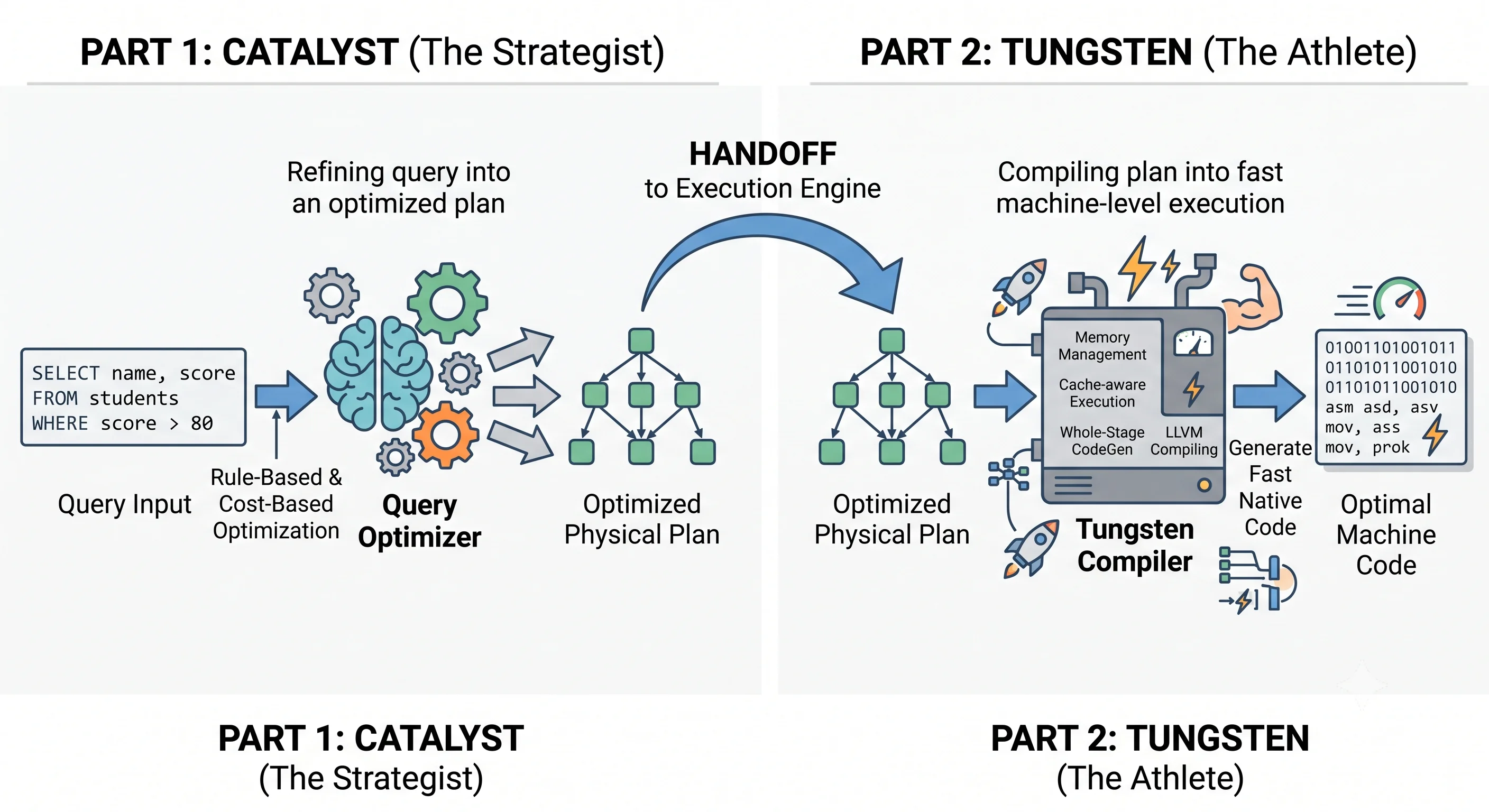
Two components are responsible:

Catalyst — the query optimizer. It takes your DataFrame/SQL code and works out the smartest plan to execute it. Think: the brilliant strategist.
Tungsten — the execution backend. It takes Catalyst's chosen plan and runs it with ruthless efficiency on the hardware. Think: the elite athlete who executes the strategy.

Catalyst decides what to do; Tungsten makes doing it fast. Together they're the reason the structured APIs beat hand-written RDD code almost every time.

Catalyst (the strategist) refines a query into an optimized plan, then hands off to Tungsten (the athlete), which compiles it into fast machine-level execution.

Catalyst: the query optimizer

Catalyst is Spark SQL's query planning and optimization engine. It's a rule-based and cost-based optimizer that takes the query you wrote and transforms it, step by step, into highly optimized executable code. Crucially, it works identically no matter which structured API you used — DataFrame code, Dataset code, or a raw SQL string all enter the same Catalyst pipeline and come out as the same optimized plan.

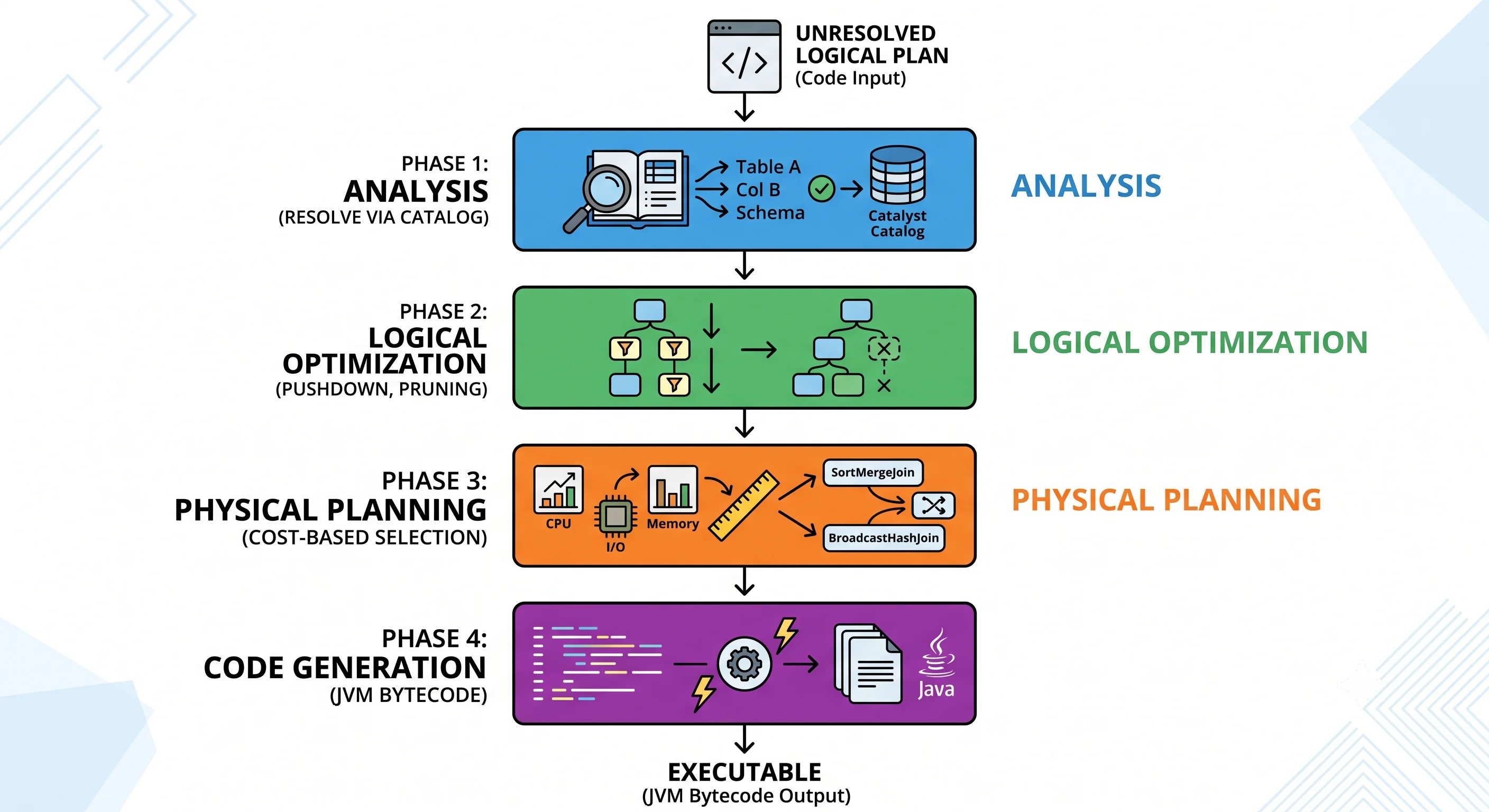
Catalyst processes every query through four distinct phases. Let's walk them in order, because each does a recognizably different job.

Analogy — planning a road trip. Catalyst is like a meticulous trip planner. First it makes sure the places you named actually exist (analysis). Then it finds smarter routes — skip the tolls, avoid the long way round (logical optimization). Then it considers concrete ways to drive it — highway vs. back roads — and picks the cheapest by time and fuel (physical planning). Finally it hands you precise turn-by-turn directions your car can follow (code generation).

Phase 1 — Analysis

Spark first parses your code into an unresolved logical plan. At this point the plan is syntactically valid but Spark doesn't yet know whether the columns and tables you named actually exist — they're just names. The Analyzer resolves them by consulting the Catalog, Spark's internal metadata repository of all known tables, columns, and their types. It checks that df.select("country") refers to a real country column of a known type, producing a resolved logical plan.

This is also why a typo in a column name surfaces as an error the moment you trigger the query (recall the DataFrame-vs-Dataset discussion in Module 04): the Analyzer couldn't resolve the name against the Catalog.

Phase 2 — Logical Optimization

Now Catalyst improves the resolved plan by applying a library of rule-based optimizations — and, where helpful, evaluating multiple candidate plans. These are the concrete rewrites we previewed in Module 06:

Predicate pushdown — move filters as close to the data source as possible so less data is read.
Projection pruning — drop columns the query never uses so they're never carried.
Constant folding — precompute constant expressions once instead of per row.
Boolean expression simplification — reduce redundant or trivially-true/false conditions.

The output is an optimized logical plan — still a description of what to compute, but a much leaner one. Note that all of this is possible only because laziness gave Catalyst the whole query to rearrange (Module 06).

Phase 3 — Physical Planning

A logical plan says what; a physical plan says how. Here Catalyst generates one or more physical plans — concrete execution strategies using Spark's physical operators. A single logical join, for example, could be executed as a broadcast hash join or a shuffle sort-merge join (Module 16), and those perform very differently.

Catalyst uses a Cost-Based Optimizer (CBO) to estimate the cost of each candidate physical plan — using statistics about data sizes — and selects the cheapest one. This is where the optimizer's decisions about joins and shuffles get made concrete.

Phase 4 — Code Generation

Finally, Catalyst hands the chosen physical plan to Project Tungsten, which compiles it into compact Java bytecode that runs directly on the JVMs across the cluster. This is the bridge to the second half of the module — and where Catalyst's plan becomes blazing-fast machine work.

Catalyst's four phases as a vertical pipeline: Analysis (resolve via the Catalog) → Logical Optimization (pushdown, pruning) → Physical Planning (cost-based selection) → Code Generation (JVM bytecode); code enters the top, executable code exits the bottom.

Seeing all four phases

You can watch Catalyst's journey with the extended form of explain() from Module 06:

result = (spark.read.parquet("/data/sales")
          .select("id", "country", "amount")
          .filter("country = 'Japan'"))

# Shows Parsed → Analyzed → Optimized logical plans, then the selected Physical plan.
result.explain(mode="extended")

Reading top to bottom, you can literally see the unresolved plan get resolved, then optimized (watch filters and projections migrate toward the source), then turned into a physical plan with concrete operators.

Project Tungsten: making the plan fast

Catalyst picks a great plan. Tungsten is what makes executing that plan approach the limits of the hardware. It attacks the two biggest sources of overhead in a JVM data engine: memory/object overhead and per-operation function-call overhead.

Off-heap, row-based binary format

Ordinary JVM programs represent each record as a Java object on the JVM heap. For billions of rows that's catastrophic: huge memory overhead per object and relentless garbage collection (GC) pauses as the JVM cleans up short-lived objects.

Tungsten sidesteps this entirely. It lays out DataFrame/Dataset rows in a compact binary format in off-heap memory — memory Spark manages directly, bypassing the JVM heap. The wins are large:

No per-object overhead — data is packed tightly as bytes, not bloated Java objects.
No GC pressure — because the data lives off-heap, the garbage collector isn't constantly scanning and pausing to reclaim it.

This binary format is also what lets a Python DataFrame match Scala performance (Module 04): the data never becomes language-specific objects; it stays as Tungsten bytes that the JVM operates on directly.

Whole-stage code generation

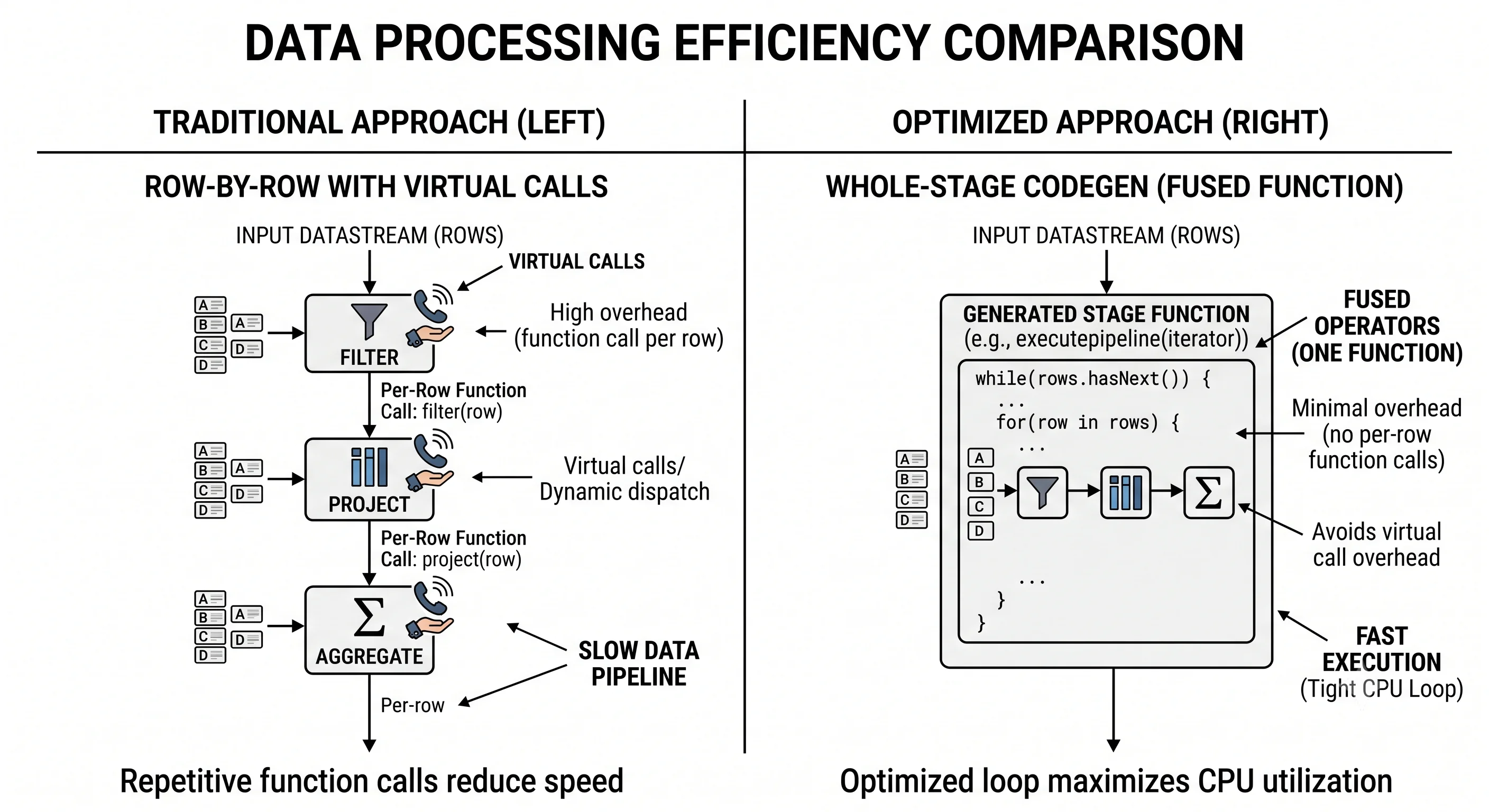
The second trick is whole-stage code generation. Normally, executing a plan means calling a separate function for each operator on each row — filter function, then project function, then next function — with a virtual function call at every step. Across billions of rows, those calls dominate the runtime.

Tungsten collapses an entire stage of operations (recall stages from Modules 02 and 07) into a single, hand-written-looking Java function. Instead of many small function calls per row, one tight loop does everything. This eliminates virtual function-call overhead and keeps intermediate values in CPU registers rather than shuffling them through memory — the kind of code you'd write by hand if you had infinite patience, generated automatically.

Analogy — an assembly line vs. one master craftsman per item. The naive approach is like passing each product down a line where a different worker performs one tiny step and hands it on — lots of handoffs (function calls), lots of waiting. Whole-stage codegen is like training a single master craftsman to perform all the steps for a product in one fluid motion at their bench, with the tools already in hand (CPU registers). No handoffs, no waiting — just one efficient pass.

Row-by-row execution with a virtual call per operator per row versus whole-stage code generation, where operators are fused into one compact function processing rows in a tight loop.

Why this module matters even though it's automatic

You don't invoke Catalyst or Tungsten — they run for you every time you use the structured APIs. So why learn them? Because they justify nearly every recommendation in this guide:

"Prefer DataFrames/SQL over RDDs" (Module 04) means "let Catalyst and Tungsten work" — RDDs bypass both.
"Avoid Python UDFs where you can" (Module 12) means "don't force data out of Tungsten's binary format into Python objects."
"Use native null and built-in functions" (Module 17) means "stay on paths Catalyst knows how to optimize."
Reading explain() (Module 06) is reading Catalyst's output.

Understanding these two engines turns a list of "best practices" into a coherent principle: stay in the structured, binary, optimizable world, and get out of Catalyst and Tungsten's way.

Key takeaways

Catalyst is Spark SQL's rule- and cost-based query optimizer; Tungsten is the execution backend that runs the optimized plan fast. Catalyst decides what; Tungsten makes doing it fast.
Catalyst runs four phases: Analysis (resolve names/types via the Catalog), Logical Optimization (predicate pushdown, projection pruning, constant folding, boolean simplification), Physical Planning (generate candidate plans, pick cheapest via the Cost-Based Optimizer), and Code Generation (compile to JVM bytecode via Tungsten).
All structured APIs (DataFrame, Dataset, SQL) enter the same Catalyst pipeline — the reason they share performance across languages.
Tungsten stores rows in a compact off-heap binary format (no per-object overhead, no GC pressure) and uses whole-stage code generation to fuse a stage's operators into one tight function (no virtual calls, values kept in CPU registers).
Inspect the whole journey with explain(mode="extended").
These engines are the reason behind most best practices: stay structured, stay in the binary format, and let Catalyst and Tungsten optimize.

Check your understanding

Put the four Catalyst phases in order and give a one-line job for each. Which phase catches a misspelled column name, and how?
Tungsten stores data off-heap in a binary format instead of as JVM objects. Name the two performance problems this solves.
In your own words, what does whole-stage code generation replace, and why is fusing a stage into one function faster than calling an operator per row?

Up next

SparkSession Getting Started — SparkSession & Getting Started. That completes the engine internals. Now we shift into Part IV — Writing PySpark, starting hands-on: creating and configuring a SparkSession, and reading data the right way — with explicit schemas instead of costly inference.