MLlib Pipelines

Part IV — Writing PySpark · Module 14 of 18 Prerequisites: DataFrame Operations, Transformations & Actions, Caching & Persistence (referenced; caching intermediate features) You will learn: how Spark does machine learning at scale with MLlib — the difference between transformers and estimators, how the Pipeline API chains preprocessing and modeling into one repeatable workflow, and the standard feature-engineering steps (indexing, encoding, vector assembly) that get raw data ready for a model.

---

Machine learning on distributed data

Everything you've learned about DataFrames pays off again here. MLlib is Spark's built-in machine learning library, and its modern API is built on DataFrames — so the same distributed, partitioned, Catalyst-optimized data structures you've used all along are exactly what you feed to a model. Training scales across the cluster just like any other Spark job.

MLlib organizes ML around a small, elegant vocabulary borrowed loosely from scikit-learn but adapted for distributed data. Learn four words — transformer, estimator, pipeline, and the fit/transform pattern — and the rest falls into place.

---

Transformers vs. estimators: the two building blocks

Every step in an MLlib workflow is one of two things:

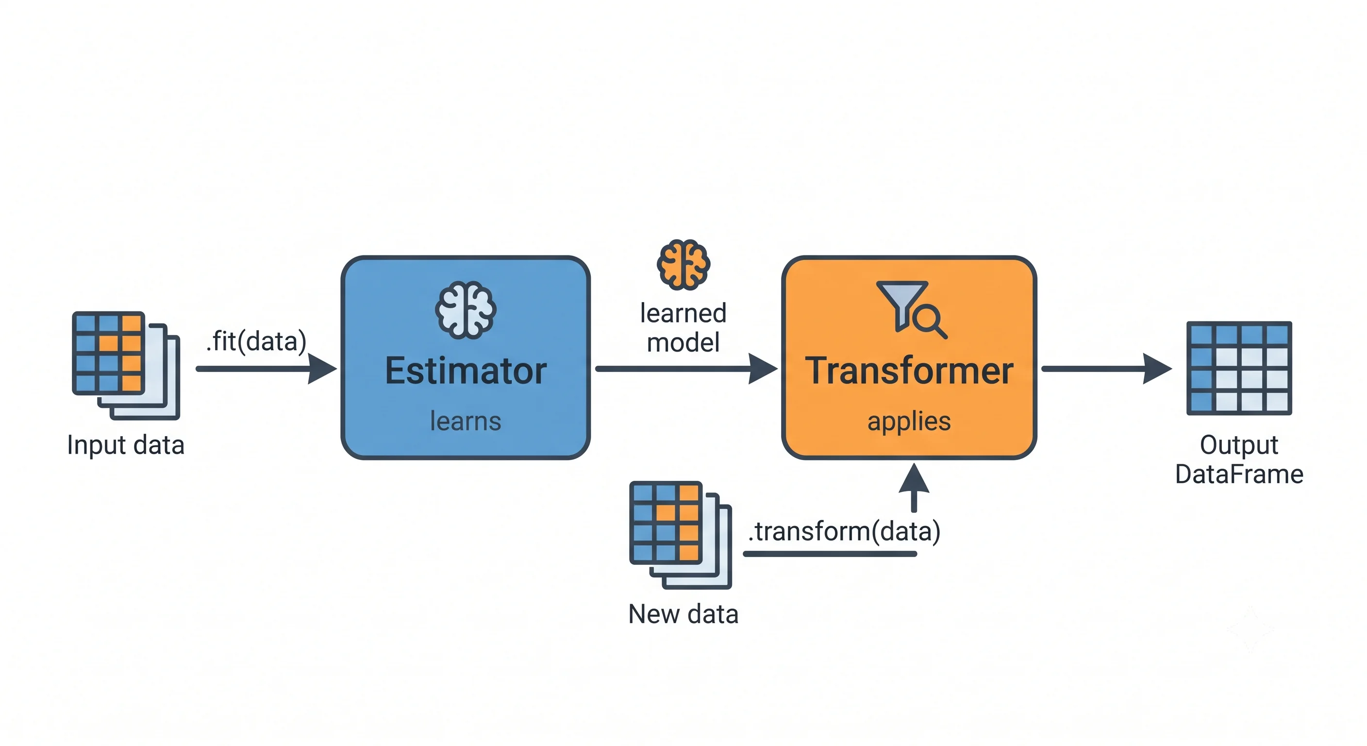
• A Transformer transforms one DataFrame into another via a .transform() method. It applies a fixed, already-known rule — no learning involved. Encoding a column, assembling features into a vector, or a trained model making predictions are all transformers.
• An Estimator learns from data via a .fit() method, and .fit() returns a transformer. An estimator is an algorithm that must look at the data first to produce something reusable — computing the categories in a column, or training a model.

The relationship is the crux: an estimator's .fit() produces a transformer. You fit to learn, then transform to apply.

Analogy — a tailor learning your measurements. An estimator is the tailor taking your measurements: they study you (.fit() on the data) and produce a pattern cut to your size. That pattern is a transformer — a fixed template that can now cut fabric (.transform()) for you again and again without re-measuring. Fitting is the one-time learning; transforming is the repeatable application.

---

The feature-engineering steps

Machine learning algorithms in MLlib expect a specific input shape: a single column, conventionally named features, holding a numeric vector for each row. Real data rarely starts that way — it has text categories, multiple separate numeric columns, and so on. So most of the work is transforming raw columns into that one features vector. Here are the standard tools, each a transformer or estimator you now recognize:

1. StringIndexer — turn categories into numbers (estimator)

Models need numbers, not strings. StringIndexer maps each distinct string category to a numeric index. It's an estimator because it must first scan the data to learn which categories exist:

from pyspark.ml.feature import StringIndexer

indexer = (StringIndexer()
           .setInputCol("day_of_week")
           .setOutputCol("day_of_week_index"))

2. OneHotEncoder — avoid fake ordering (transformer)

A raw index (Monday=0, Tuesday=1, …) accidentally implies an order and magnitude that isn't real — a model might think "Sunday (6) > Monday (0)." OneHotEncoder converts each index into a sparse vector with a single 1, removing that false ordering:

from pyspark.ml.feature import OneHotEncoder

encoder = (OneHotEncoder()
           .setInputCol("day_of_week_index")
           .setOutputCol("day_of_week_encoded"))

3. VectorAssembler — combine into one features column (transformer)

Finally, VectorAssembler gathers all your prepared feature columns — numeric ones plus the encoded categoricals — into the single features vector the model expects:

from pyspark.ml.feature import VectorAssembler

assembler = (VectorAssembler()
             .setInputCols(["UnitPrice", "Quantity", "day_of_week_encoded"])
             .setOutputCol("features"))

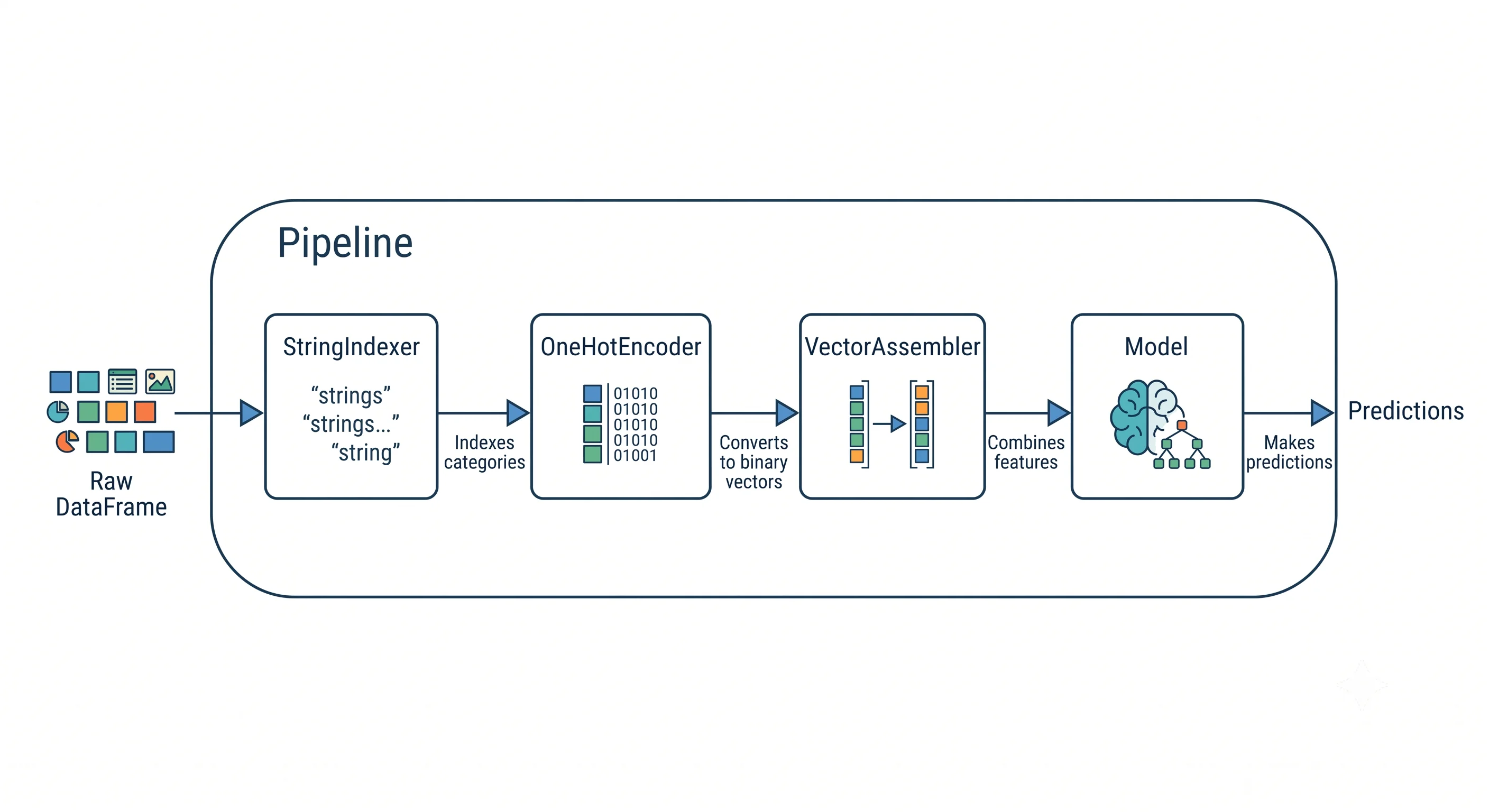
The pattern to notice: raw columns → indexed → encoded → assembled into features. Nearly every MLlib workflow walks this same path.

---

The Pipeline: chaining it all into one repeatable workflow

You could call .fit() and .transform() on each step by hand, threading the output of one into the input of the next. But that's tedious and — more dangerously — easy to get subtly wrong (especially the train/test discipline below). The Pipeline solves this by packaging an ordered list of stages into a single estimator.

A Pipeline is itself an estimator: you .fit() the whole pipeline once, and it runs each stage in order, fitting the estimators and applying the transformers, producing a single fitted PipelineModel (a transformer) that encapsulates the entire workflow.

from pyspark.ml import Pipeline

# Package all preprocessing stages into one ordered workflow.
pipeline = Pipeline().setStages([indexer, encoder, assembler])

# Fit the whole pipeline once — every stage is fit/applied in sequence.
pipeline_model = pipeline.fit(train_df)

# Apply the fitted pipeline to produce the model-ready features column.
prepared_train = pipeline_model.transform(train_df)

The huge benefit: the same fitted pipeline can be applied to new data — validation sets, test sets, or tomorrow's production data — guaranteeing the identical preprocessing every time. No drift between how you prepared training data and how you prepare live data.

Analogy — an assembly line for data. A pipeline is a factory line where each station does one job — index here, encode there, assemble at the end — and every item passes through the stations in the same order. Once the line is set up (fit), any raw material you feed in comes out as a finished, consistently-prepared product. New batches get the exact same treatment, so results are reproducible.

---

Training a model and the train/test split

Modeling algorithms are just more pipeline stages. A classifier or clustering algorithm is an estimator; fitting it yields a model (a transformer) that makes predictions. First, the non-negotiable discipline: split your data so you evaluate on data the model never saw.

from pyspark.ml.clustering import KMeans

# Hold out a test set the model never trains on (reproducible with a seed).
train_df, test_df = data.randomSplit([0.8, 0.2], seed=42)

# A model is an estimator too — add it as the final pipeline stage.
kmeans = KMeans().setK(20).setSeed(1).setFeaturesCol("features")

full_pipeline = Pipeline().setStages([indexer, encoder, assembler, kmeans])

model = full_pipeline.fit(train_df)          # fit preprocessing + model together
predictions = model.transform(test_df)        # apply the SAME steps to unseen data
predictions.show(5)

Because the model sits inside the pipeline, the test set flows through the exact same indexing, encoding, and assembly as the training set — the pipeline enforces consistency for you.

Cache intermediate features when you iterate

Model training is often iterative — an algorithm sweeps over the same prepared features many times, and you may retrain repeatedly while tuning. Recall from Module 06 that Spark recomputes a DataFrame from scratch on every action, and from Module 15 that caching avoids that. Prepared training features are a textbook case:

prepared_train = pipeline_model.transform(train_df)
prepared_train.cache()          # keep features in memory across training iterations
prepared_train.count()          # materialize the cache now (an action — see Module 15)

Without caching, every training iteration would re-run the whole indexing/encoding/assembly chain. With it, that expensive preparation happens once and every iteration reads from memory. (Full caching guidance is Module 15.)

---

A note on ensembles: the wisdom of the crowd

One MLlib idea is worth calling out because it's both powerful and intuitive: ensembles, like the Random Forest. Instead of trusting a single decision tree — which can easily overfit and be brittle — a Random Forest trains many trees on different slices of the data and combines their votes.

Analogy — guessing M&Ms in a jar. Ask one person to guess how many M&Ms are in a jar and they'll likely be off. But average the guesses of a hundred people and the result lands remarkably close to the truth — individual errors cancel out. A Random Forest works the same way: each tree is a "weak" individual guesser, but combining a crowd of them yields a robust, accurate prediction. This is the wisdom of the crowd, and it's why ensembles are among the most reliable everyday ML models.

---

Key takeaways

• MLlib is Spark's ML library, built on DataFrames, so models train on the same distributed, optimized data structures you've used throughout.
• Every step is a transformer (.transform(), applies a known rule) or an estimator (.fit(), learns from data). Crucially, an estimator's .fit() returns a transformer — fit to learn, transform to apply.
• Standard feature engineering flows raw → StringIndexer → OneHotEncoder → VectorAssembler → single features vector that models expect.
• A Pipeline packages ordered stages into one estimator; .fit() yields a PipelineModel that applies the identical preprocessing to any new data — reproducible and drift-free.
• Always split into train/test (randomSplit) and let the pipeline push both through the same steps; cache prepared features when training iteratively (Module 15).
• Ensembles like Random Forests combine many weak models into a strong one — the "wisdom of the crowd."

---

Check your understanding

1. What's the essential difference between a transformer and an estimator, and what does an estimator's .fit() return?
2. Why do we one-hot encode an indexed category instead of feeding the raw integer index straight to the model?
3. Why is wrapping preprocessing and the model in a single Pipeline safer than applying each step to the train and test sets by hand?

---

Up next

Caching & Persistence — Caching & Persistence. That completes Part IV. We enter Part V — Running It Well, starting with the caching we kept invoking: when it genuinely pays off, when it backfires, the storage levels, and why you must materialize a cache to make it real.