Structured Streaming

Part IV — Writing PySpark · Module 13 of 18 Prerequisites: DataFrame Operations, Transformations & Actions, SparkSession Getting Started You will learn: how Spark applies the same DataFrame API to unbounded, real-time data; the mental model of a stream as an "infinite table"; how to read a stream (readStream), aggregate over event-time windows, and write results (writeStream); plus output modes and triggers.

---

The big idea: a stream is just an unbounded table

Every module so far worked on a finite dataset — a file, a table, a fixed collection of rows. But much of the world's data arrives continuously: clickstreams, sensor readings, transactions, log lines. Structured Streaming is Spark's engine for processing that never-ending data.

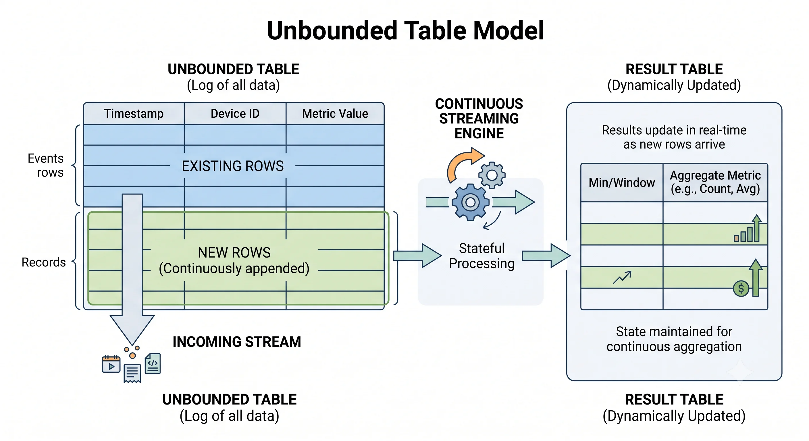
Its central, beautiful idea is this: treat a live data stream as a table that is continuously being appended to. New data arriving is just new rows added to the bottom of an (infinitely growing) input table. And once you think of a stream as a table, a profound consequence follows:

You use the exact same DataFrame API you already know. select, filter, groupBy, agg — the operations from Module 10 work unchanged. You write essentially the same code whether the data is a static file or a live firehose. Spark handles the hard parts of incremental, continuous computation underneath.

Analogy — a ledger that never closes. A batch dataset is a finished accounting ledger: all the entries are written, you total the columns, done. A stream is a ledger that stays open forever — new lines are added around the clock. Structured Streaming lets you ask "what's the running total per account?" against that open ledger, and it keeps the answer continuously up to date as new lines appear. You ask the question once; Spark keeps answering it.

---

Reading a stream: readStream

Where a batch job uses spark.read, a streaming job uses spark.readStream — nearly identical in shape. Here we read a directory where new CSV files keep landing; each new file becomes new rows in the unbounded table:

from pyspark.sql.types import StructType, StructField, StringType, DoubleType, TimestampType

# Streaming sources require an EXPLICIT schema — there's no finite data to infer from.
schema = StructType([
    StructField("InvoiceNo",   StringType(),    True),
    StructField("CustomerId",  StringType(),    True),
    StructField("UnitPrice",   DoubleType(),    True),
    StructField("Quantity",    DoubleType(),    True),
    StructField("InvoiceDate", TimestampType(), True),
])

stream_df = (spark.readStream
             .schema(schema)                       # mandatory for streams
             .option("maxFilesPerTrigger", 1)      # process one new file per trigger (demo pacing)
             .format("csv")
             .option("header", "true")
             .load("/data/retail/by-day/*.csv"))

Two things to flag:

• A schema is required. With batch data Spark could infer a schema by scanning the data (Module 09) — but a stream has no finite end to scan, so you must always supply the schema explicitly. (Another reason the explicit-schema habit from Module 09 pays off.)
• The result, stream_df, is a streaming DataFrame. It looks and behaves like a normal DataFrame, but it's backed by the unbounded table.

---

Transforming a stream: the same operations, plus event-time windows

You transform a streaming DataFrame with the familiar API. The one genuinely new concept is the event-time window — because with continuous data, you usually want to aggregate over time buckets ("total sales per day," "clicks per 5-minute window") rather than over the whole infinite table.

Event time means the timestamp on the data itself (when the event actually happened), not when Spark processed it. The window() function groups rows into time buckets based on that column:

from pyspark.sql.functions import col, window

# Total spend per customer, bucketed into 1-day event-time windows.
purchases_per_day = (stream_df
    .selectExpr(
        "CustomerId",
        "(UnitPrice * Quantity) AS total_cost",
        "InvoiceDate")
    .groupBy(
        col("CustomerId"),
        window(col("InvoiceDate"), "1 day"))    # <-- event-time window
    .sum("total_cost"))

Notice this is an ordinary groupBy(...).sum(...) — a wide transformation just like Module 10 — with window(col("InvoiceDate"), "1 day") as one of the grouping keys. Spark maintains these per-window aggregates incrementally as new data streams in, updating the results without recomputing from scratch. (Real pipelines add watermarks to bound how long Spark waits for late-arriving events; that's a next-step topic beyond this introduction.)

---

Writing a stream: writeStream, output modes, and triggers

A batch job ends with an action like show() or write.save(). A streaming job instead ends with writeStream, which starts a continuous query that runs indefinitely, updating its output as data flows.

# Write the running results to an in-memory table you can query (handy for demos/debugging).
query = (purchases_per_day.writeStream
         .format("memory")                 # sink: an in-memory table
         .queryName("purchases")           # name to query via spark.sql
         .outputMode("complete")           # emit the full updated result each time
         .start())                         # launch the continuous query

# The stream now runs in the background; query its current state anytime:
spark.sql("SELECT * FROM purchases ORDER BY sum(total_cost) DESC LIMIT 5").show()

Two streaming-specific choices appear here: output mode and (implicitly) the trigger.

Output modes — what to emit each time

Because the result table keeps changing, you must tell Spark which rows to push to the sink on each update:

• append — only brand-new rows since the last trigger. Best for streams where past rows never change (e.g., simple filtering/transformation with no aggregation).
• complete — the entire updated result table every time. Required for aggregations where totals keep shifting (like our per-window sums), but only feasible when the result stays reasonably small.
• update — only the rows that changed since the last trigger. A middle ground — efficient for aggregations without re-emitting everything.

Triggers — how often to process

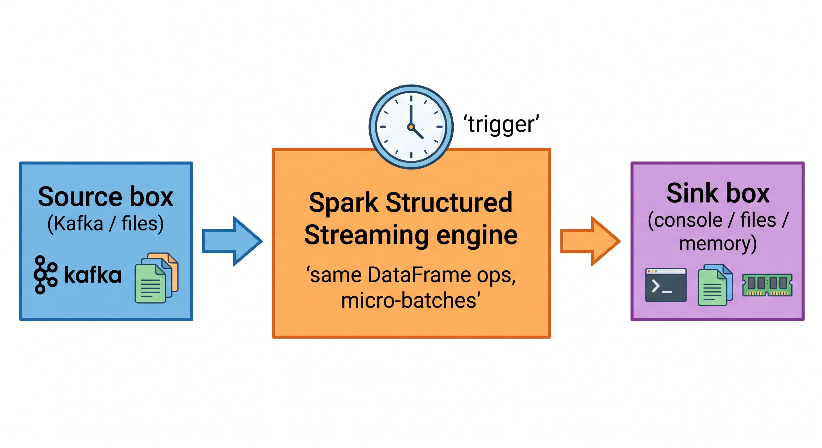
The trigger controls the cadence — how often Spark checks for new data and produces a batch of output. By default Spark processes data as fast as it can, in micro-batches (small batches processed back-to-back, which is how Structured Streaming achieves near-real-time results). You can also set a fixed interval:

from pyspark.sql.streaming import Trigger  # illustrative

query = (purchases_per_day.writeStream
         .format("console")
         .outputMode("update")
         .trigger(processingTime="10 seconds")   # produce output every 10 seconds
         .start())

Common sources and sinks

Structured Streaming reads from and writes to many systems. The most common sources are files (a directory of arriving files) and Apache Kafka (a distributed, fault-tolerant buffer of record streams — the workhorse of real-time pipelines). Common sinks include files, Kafka, the console (debugging), and the in-memory table shown above.

---

Why "same API" is such a big deal

It's worth pausing on the payoff. Before Structured Streaming, real-time systems forced developers to learn a completely different, lower-level programming model — manually managing state, handling failures, tracking what had already been processed, and stitching together "plumbing." It was error-prone and had little in common with batch code.

Structured Streaming collapses that gap. Because a stream is modeled as an unbounded table and you use the same DataFrame operations, the batch logic you already wrote is most of the way to a streaming job. The same Catalyst optimizer (Module 08) plans it; the same concepts (transformations, actions-turned-queries, shuffles for windowed aggregations) apply. Spark takes on the genuinely hard parts — incremental computation, fault-tolerant state, exactly-once processing — so you don't hand-build them. This is the "unified engine" promise from Module 01 delivered in full: one API, batch and streaming.

---

Key takeaways

• Structured Streaming models a live stream as an unbounded table that's continuously appended to — so you process it with the same DataFrame API as batch data.
• Read with spark.readStream (a schema is mandatory — no finite data to infer from); the result is a streaming DataFrame.
• Aggregate over time using event-time windows via window(col("timestamp"), "duration") inside a groupBy — Spark maintains the aggregates incrementally.
• Write with writeStream ... .start(), which launches a continuous query. Choose an output mode — append (new rows), complete (full result, for aggregations), or update (changed rows) — and a trigger (cadence; default is micro-batches).
• Common sources/sinks include files, Kafka (a distributed buffer), the console, and in-memory tables.
• The headline benefit: the same code and engine serve batch and streaming, so Spark handles incremental, fault-tolerant, near-real-time computation for you.

---

Check your understanding

1. Explain the "unbounded table" model and why it lets you reuse the batch DataFrame API on streams.
2. Why must you always supply an explicit schema to readStream, when batch reads can sometimes infer one?
3. You're computing a running per-day total that keeps changing as data arrives. Which output mode fits, and why wouldn't append work here?

---

Up next

MLlib Pipelines — MLlib & Pipelines. We've now covered batch and streaming data processing. Next we use Spark for machine learning at scale: assembling repeatable workflows with transformers, estimators, and the Pipeline API — indexing categories, encoding features, assembling vectors, and training a model.