Joins & Broadcast

Part V — Running It Well · Module 16 of 18 Prerequisites: The Shuffle (essential — joins are a prime shuffle source), Transformations & Actions, Partitions & Parallelism You will learn: why joins are so shuffle-heavy, the two join strategies Spark chooses between — the shuffle sort-merge join and the broadcast hash join — how to trigger a broadcast (and tune its threshold), and how bucketing can eliminate the join shuffle for two large tables entirely.

---

Why joins deserve their own module

Joining is everywhere in data work — enrich transactions with customer details, attach product names to order IDs, combine fact and dimension tables. It's also, as we flagged in Module 07, one of the most expensive things you can ask Spark to do, because matching rows on a key generally requires a shuffle to bring matching keys together.

The good news: Spark has more than one way to perform a join, and choosing the right strategy — or nudging Spark toward it — can turn an agonizingly slow join into a fast one. This module is about that choice.

---

The default: shuffle sort-merge join (SMJ)

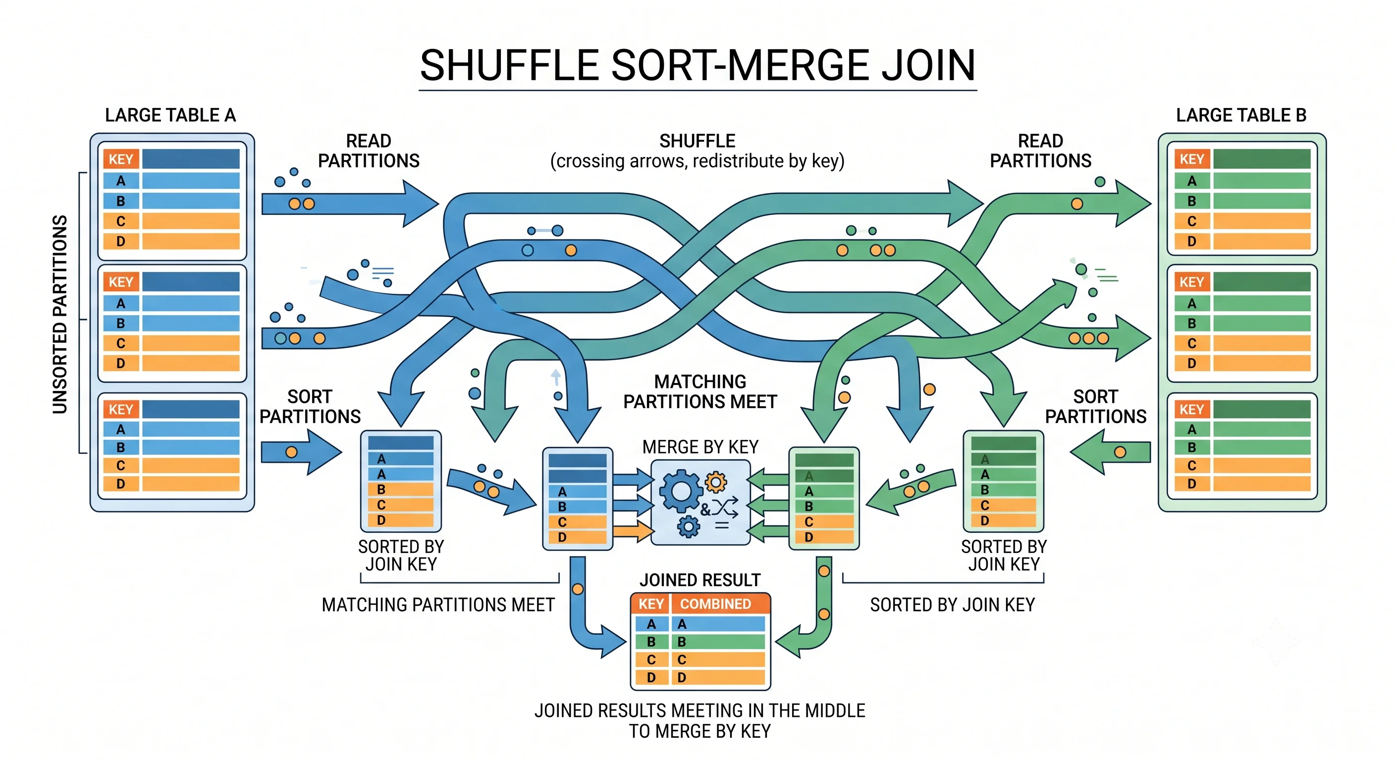
When you join two large tables on a key, Spark's default strategy is the shuffle sort-merge join (SMJ). It works in the shape you'd expect from Module 07's four-phase shuffle:

1. Shuffle both tables so that rows with the same join key land in the same partition on the same executor (an Exchange for each input).
2. Sort each partition by the join key.
3. Merge — walk the two sorted partitions together, matching rows with equal keys.

It's a robust, general-purpose strategy that works for any two tables. But notice the cost: both datasets are shuffled across the network and sorted. For two big tables that's a lot of movement — the join is doing the most expensive operation, twice over.

Analogy — merging two sorted guest lists. Two event organizers each have a pile of unsorted RSVP cards. To find people on both lists, they first re-sort their piles alphabetically (sort), make sure both are using the same alphabetical buckets (shuffle), then walk down the two sorted piles in lockstep, matching names (merge). Effective, but re-sorting and re-bucketing both big piles is the slow part.

---

The fast path: broadcast hash join (BHJ)

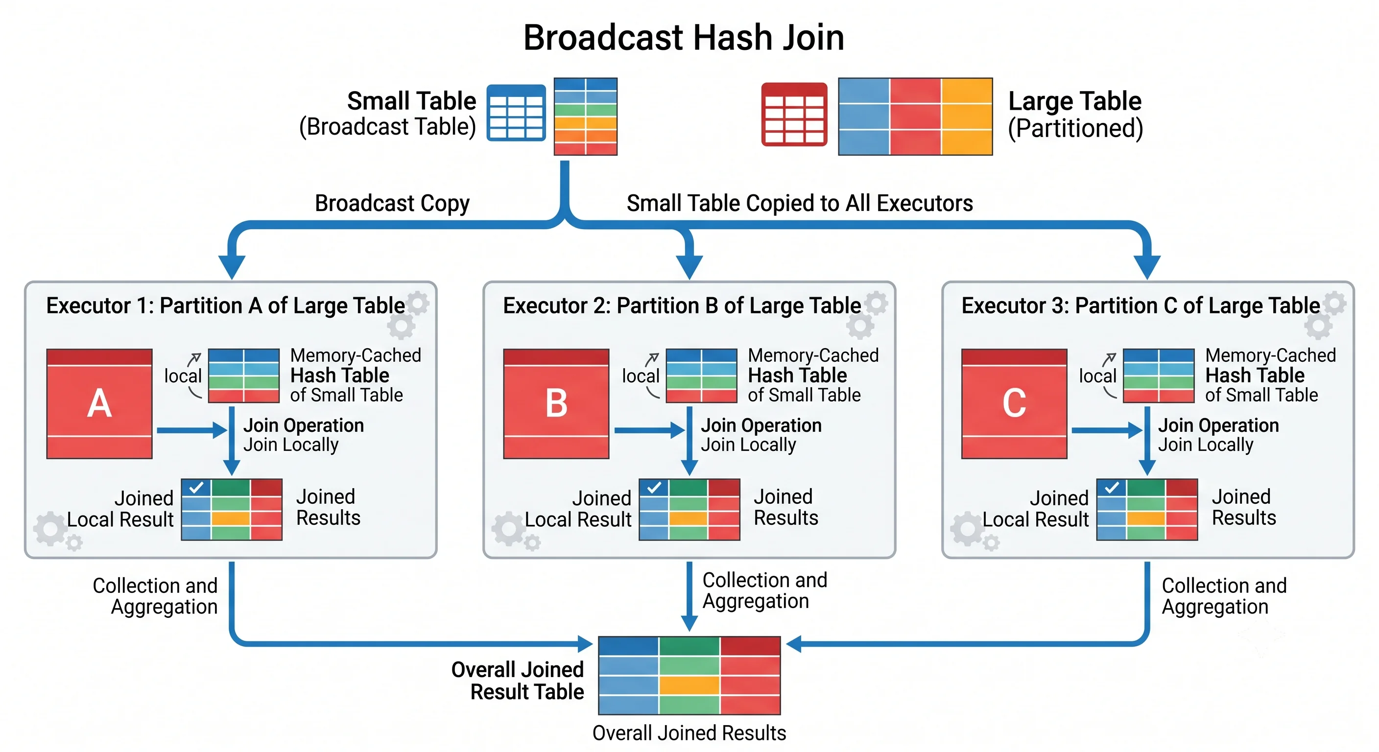
Here's the key insight. Very often you're not joining two equally large tables — you're joining one huge table (a fact table: millions of transactions) with one small table (a lookup/dimension: a few thousand product names). In that lopsided case, shuffling the giant table is wasteful, and there's a much better way: the broadcast hash join (BHJ).

Instead of shuffling both tables, Spark takes the small table and broadcasts a full copy of it to every executor. Now each executor already has the entire lookup table in memory, so it can join its local partitions of the big table without moving the big table at all. No shuffle of the large dataset, no sort — every executor works locally.

from pyspark.sql.functions import broadcast

# Explicitly hint Spark to broadcast the small dimension table.
joined = large_fact_df.join(broadcast(small_dim_df), "product_id")

The broadcast() hint tells Spark "this side is small — ship it everywhere." The payoff is enormous: you replace two big shuffles with one small broadcast. For the common huge-joins-small pattern, BHJ is the single most effective join optimization (it was the top shuffle-killer in Module 07's toolkit).

Analogy — a shared cheat sheet. Suppose 100 clerks each have a stack of order forms listing product codes, and you need the product names. The slow way (SMJ) is to gather and re-sort everyone's forms together. The fast way (BHJ) is to hand every clerk a copy of the small code→name sheet. Now each clerk fills in names from their own desk, in parallel, with no gathering at all. The cheat sheet is the broadcast; it's cheap because it's small enough to copy everywhere.

---

Controlling broadcasts: the threshold

Spark will often perform a broadcast join automatically when it can tell one side is small enough. The cutoff is governed by a configuration:

# Tables estimated smaller than this are auto-broadcast. Default: 10 MB.
spark.conf.set("spark.sql.autoBroadcastJoinThreshold", 10 * 1024 * 1024)   # 10 MB

# Raise it if your executors have memory to spare and your lookup tables are larger:
spark.conf.set("spark.sql.autoBroadcastJoinThreshold", 50 * 1024 * 1024)   # 50 MB

# Disable auto-broadcast entirely by setting it to -1:
spark.conf.set("spark.sql.autoBroadcastJoinThreshold", -1)

• The default threshold is 10 MB — tables Spark estimates to be smaller are broadcast automatically.
• If your executors have ample memory, raising the threshold (say to 50–100 MB) lets Spark broadcast somewhat larger lookup tables and skip more shuffles.
• Setting it to -1 disables automatic broadcasting.

You can always force the decision yourself with the explicit broadcast() hint shown earlier, which overrides the automatic estimate.

The essential caution — don't broadcast something big. A broadcast sends a full copy of the table to every executor and stages it through the driver. If you broadcast a table that's actually large, you can exhaust executor memory or blow up the driver (the same driver out-of-memory risk from Module 02). Broadcast only genuinely small tables. When in doubt, check the size before hinting.

---

Eliminating the shuffle for two large tables: bucketing

Broadcast joins solve the huge-joins-small case. But what if both tables are large? You can't broadcast either one. Are you stuck paying for a full sort-merge shuffle every time? Not if you plan ahead with bucketing.

The SMJ is slow because it shuffles and sorts at query time, every time. Bucketing moves that cost to write time, once. When you write a table, you pre-partition and pre-sort it into a fixed number of buckets on the join key, saved as a managed table (typically in Parquet):

# Write both tables bucketed and sorted on the join key, ONCE.
(users_df
 .write
 .bucketBy(8, "user_id")          # 8 buckets, hashed on user_id
 .sortBy("user_id")
 .saveAsTable("users_bucketed"))

(orders_df
 .write
 .bucketBy(8, "user_id")          # SAME bucket count and key
 .sortBy("user_id")
 .saveAsTable("orders_bucketed"))

# Now this join needs NO shuffle — matching keys are already colocated & sorted.
result = spark.table("users_bucketed").join(spark.table("orders_bucketed"), "user_id")

Because both tables are already bucketed by the same key into the same number of buckets, matching keys are guaranteed to be in corresponding buckets, already sorted. Spark can read the pre-sorted buckets and merge them directly — the expensive Exchange (shuffle) and Sort phases vanish from the query. You paid that cost once, at write time, and every subsequent join is fast.

The trade-off: bucketing requires foresight (you must write the data bucketed on the key you'll join by) and works only when both tables share the same bucketing scheme. It shines for large tables joined repeatedly on a stable key — precompute the layout once, reap fast joins forever after.

---

Choosing a join strategy

A quick decision guide:

Situation	Best strategy	Why
Huge table ⋈ small lookup	Broadcast hash join	Copy the small side everywhere; don't shuffle the big one
Two large tables, one-off join	Shuffle sort-merge join (default)	Robust; no precomputation available
Two large tables, joined repeatedly on a stable key	Bucketing	Pay the shuffle/sort once at write time, then join shuffle-free

And the always-applicable habits from Module 07 still help: filter before joining to shrink both sides, and make sure your join keys use Spark's native null handling rather than dummy values (Module 17).

---

Key takeaways

• Joins are shuffle-heavy because matching rows on a key usually requires bringing those keys together across the cluster.
• The default shuffle sort-merge join (SMJ) shuffles and sorts both tables, then merges — robust but expensive for two large inputs.
• A broadcast hash join (BHJ) sends a full copy of a small table to every executor so the large table is joined locally with no shuffle — the best optimization for the common huge-⋈-small case. Trigger it with the broadcast() hint.
• Auto-broadcast is controlled by spark.sql.autoBroadcastJoinThreshold (default 10 MB; raise for more broadcasting, -1 to disable). Never broadcast a large table — it risks executor/driver OOM.
• For two large tables joined repeatedly, bucketing (pre-partition + pre-sort on the join key at write time via bucketBy) eliminates the query-time shuffle and sort entirely.
• General habits still apply: filter early, and use native nulls in join keys.

---

Check your understanding

1. Why does the default sort-merge join get expensive when both tables are large? Name the two costly phases it applies to each table.
2. You join a 3 TB events table with a 4 MB country-code lookup and it's slow. What strategy fixes it, and why does it avoid shuffling the big table?
3. Two large tables are joined on user_id in a nightly job. What one-time technique would make every future run's join shuffle-free, and what's the catch?

---

Up next

Performance Tuning — Performance Tuning. We've covered individual levers (partitions, caching, joins). Next we assemble the full tuning playbook: shuffle partitions, Adaptive Query Execution, dynamic allocation, coalesce vs. repartition, avoiding driver OOM, the small-file problem, and the native-null rule — the checklist for diagnosing and fixing a slow job.