DataFrame Operations

Part IV — Writing PySpark · Module 10 of 18 Prerequisites: SparkSession Getting Started, Transformations & Actions (transformations vs. actions), RDDs, DataFrames, Datasets You will learn: the everyday DataFrame toolkit you'll use in almost every PySpark job — selecting, filtering, grouping, aggregating, ordering, and adding/renaming/dropping columns — plus how col() and expr() let you write expressions, and why chaining these transformations is the idiomatic Spark style.

---

The daily toolkit

If Modules 01–08 were the theory and Module 09 got you a loaded DataFrame, this module is the workbench. Almost every real pipeline is built from a small set of operations applied over and over: pick columns, keep rows, group, aggregate, sort, and reshape columns. Master these and you can express the majority of data-wrangling tasks.

Everything here is a transformation (Module 05) unless we explicitly call show() — which means it's lazy and returns a new DataFrame, leaving the original untouched (Module 05's immutability). Keep that in mind: every method below hands you back a fresh DataFrame to chain onto.

For the examples, imagine a flights DataFrame df with columns date, delay, distance, origin, destination.

---

Referring to columns: col() and expressions

Before the operations, one foundational idea: how do you name a column in code? PySpark gives you a few interchangeable ways, and you'll see all of them in the wild:

from pyspark.sql.functions import col, expr

df.select("delay")            # by string name — simplest
df.select(col("delay"))       # via col() — needed when you build expressions
df.select(df["delay"])        # bracket access on the DataFrame

Plain strings are fine for simply naming a column. But the moment you want to compute with a column — compare it, do arithmetic, chain conditions — you need a Column object, which is what col() gives you:

# col() produces a Column you can build expressions on:
df.filter(col("delay") > 60)
df.withColumn("delay_hours", col("delay") / 60)

There's also expr(), which lets you write a SQL-like expression as a string — handy for anything you'd find easier to say in SQL:

# expr() evaluates a SQL expression string into a Column.
df.withColumn("long_haul", expr("distance > 1000"))
df.selectExpr("origin", "delay", "delay / 60 AS delay_hours")   # selectExpr = select + expr

Use whichever reads most clearly. col() for programmatic expressions, expr()/selectExpr() when a SQL phrasing is more natural. They all end up as the same Catalyst expressions under the hood (Module 08).

---

select() — choose columns (projection)

select() picks which columns to keep. In relational terms this is projection, and it's often the first thing you do to trim a wide table down to what you need (which also helps Catalyst prune columns — Module 06):

# Keep only the columns you care about
df.select("origin", "destination", "delay").show(5)

# Compute new columns inline while selecting
df.select(
    col("origin"),
    col("delay"),
    (col("delay") / 60).alias("delay_hours")    # .alias() names the new column
).show(5)

.alias() is how you name a computed column — without it, Spark generates an ugly auto-name like (delay / 60).

---

filter() / where() — choose rows (selection)

filter() keeps only the rows matching a condition. In relational terms this is selection. where() is a perfect synonym — identical behavior, pick whichever reads better (SQL users often prefer where):

# These two lines are exactly equivalent
df.filter(col("delay") > 60).show(5)
df.where(col("delay") > 60).show(5)

# Combine conditions with & (and), | (or), ~ (not) — parenthesize each clause!
df.filter((col("delay") > 60) & (col("origin") == "SFO")).show(5)

Common gotcha: in PySpark you combine conditions with &, |, ~ (not Python's and/or/not), and each condition must be wrapped in parentheses because of operator precedence. (col("delay") > 60) & (col("origin") == "SFO") — forget the parentheses and you'll get a confusing error.

Remember predicate pushdown from Module 06: filtering early in your chain lets Spark read and move less data. Filter first, then do expensive work.

---

groupBy() + agg() — summarize

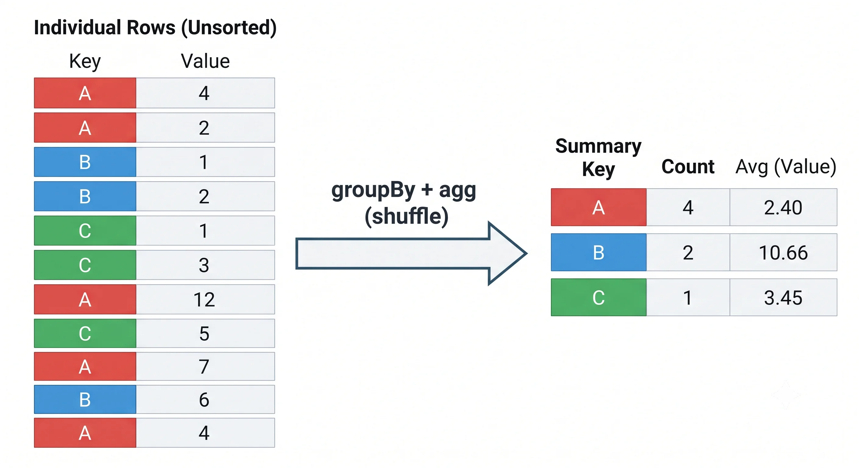
Grouping collapses many rows into per-group summaries — counts, sums, averages. This is a wide transformation (Module 05): it triggers a shuffle (Module 07), because all rows sharing a group key must come together.

from pyspark.sql.functions import count, avg, sum, max, min

# Count flights per origin
df.groupBy("origin").count().show()

# Multiple aggregations at once with agg()
(df.groupBy("origin")
   .agg(
       count("*").alias("num_flights"),
       avg("delay").alias("avg_delay"),
       max("delay").alias("worst_delay"))
   .show())

agg() is the general form — it lets you compute several aggregates in one pass and name each with .alias(). The aggregate functions (count, sum, avg, min, max, and many more) come from pyspark.sql.functions.

---

orderBy() / sort() — arrange rows

orderBy() (synonym: sort()) sorts the result. Also a wide transformation — a global sort requires a shuffle:

from pyspark.sql.functions import col, desc

# Ascending by default
df.orderBy("delay").show(5)

# Descending — two equivalent styles
df.orderBy(col("delay").desc()).show(5)
df.orderBy(desc("delay")).show(5)

# Sort by multiple columns
df.orderBy(col("origin").asc(), col("delay").desc()).show(5)

Because sorting is a shuffle, don't sort "just in case" — sort only when you actually need ordered output (echoing Module 07's advice to avoid needless wide operations).

---

Reshaping columns: withColumn, withColumnRenamed, drop

These three are the workhorses for shaping a DataFrame's columns. Each returns a new DataFrame — immutability in action (Module 05).

withColumn() — add or replace a column

from pyspark.sql.functions import expr, col

# Add a new column
df2 = df.withColumn("delay_hours", col("delay") / 60)

# Add a conditional column using a SQL CASE expression via expr()
df3 = df2.withColumn(
    "status",
    expr("CASE WHEN delay <= 10 THEN 'On-time' ELSE 'Delayed' END")
)

# If the column name already exists, withColumn REPLACES it
df4 = df3.withColumn("delay", col("delay").cast("double"))   # change delay's type

withColumn(name, expression) adds a column called name; if that name already exists, it overwrites it (a handy way to transform a column in place, like casting its type).

withColumnRenamed() — rename a column

renamed = df.withColumnRenamed("delay", "ResponseDelayedMins")

drop() — remove columns

trimmed = df.drop("distance")                 # drop one
trimmer = df.drop("distance", "destination")  # drop several

Immutability reminder: none of these mutate df. df.drop("distance") doesn't remove the column from df — it returns a new DataFrame without it. If you write df.drop("distance") and then keep using df, the column is still there. Assign the result (df = df.drop("distance")) or chain it.

---

Chaining: the idiomatic Spark style

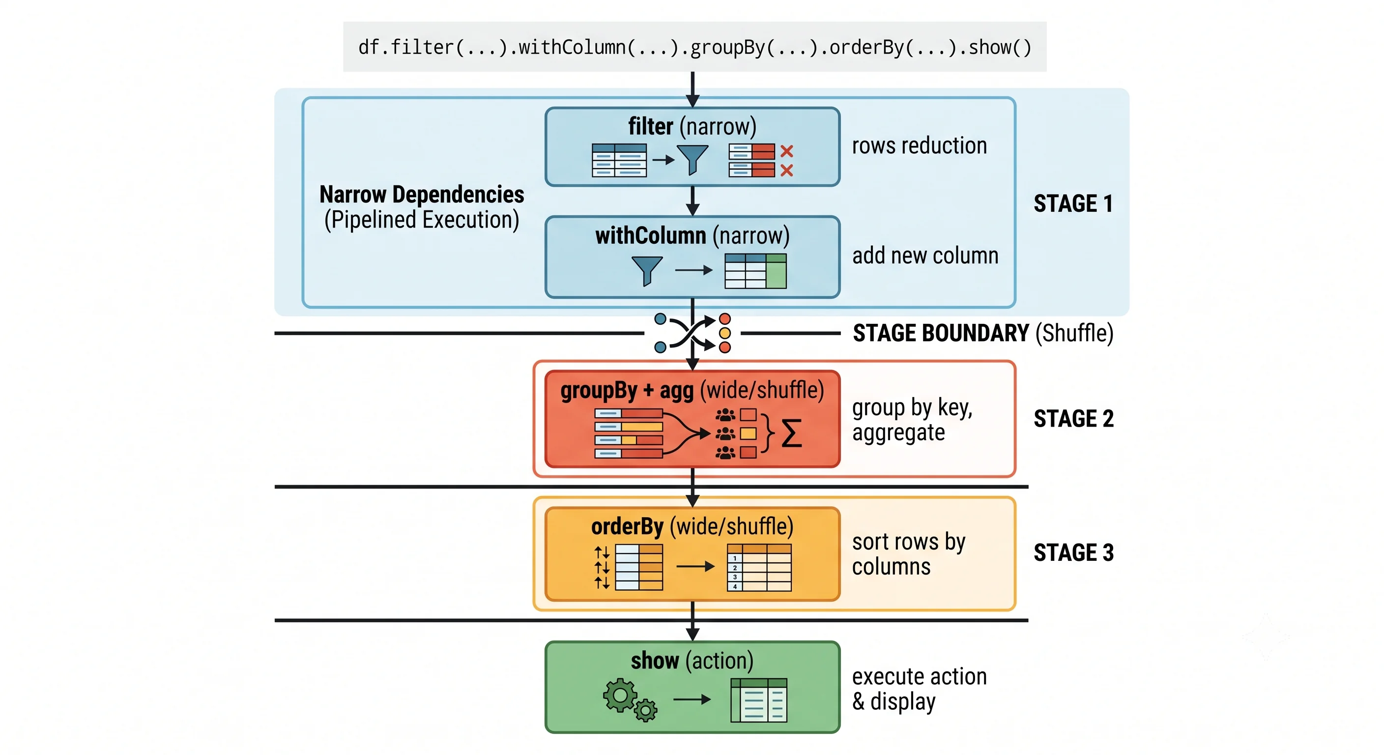
Because every transformation returns a new DataFrame, the natural way to write PySpark is to chain operations into a single fluent expression, wrapped in parentheses for readability. This reads top-to-bottom like a description of your intent:

from pyspark.sql.functions import col, count, expr

result = (df
          .filter(col("delay") > 0)                                    # keep delayed flights
          .withColumn(                                                 # classify severity
              "severity",
              expr("CASE WHEN delay > 120 THEN 'Severe' ELSE 'Minor' END"))
          .groupBy("origin", "severity")                               # summarize (shuffle)
          .agg(count("*").alias("num_flights"))                        # count per group
          .orderBy(col("num_flights").desc()))                         # sort (shuffle)

result.show(20, truncate=False)   # the single ACTION that runs the whole chain

Read that chain and notice how it maps onto everything from Part III: a narrow filter and withColumn (pipelined, no shuffle), then a groupBy and orderBy (each a wide transformation / shuffle / stage boundary), and finally one action (show) that triggers the whole lazily-built plan. The code you write here is exactly the plan Catalyst optimizes and Tungsten executes.

Style tip: wrap the chain in parentheses and put one operation per line. It's readable, diff-friendly, and lets you comment each step — the de facto convention in professional PySpark codebases.

---

Key takeaways

• The everyday toolkit: select (choose columns / projection), filter/where (choose rows / selection), groupBy+agg (summarize), orderBy/sort (arrange), and withColumn/withColumnRenamed/drop (reshape columns).
• Refer to columns with a string, col() (for building expressions), or expr()/selectExpr() (SQL-style expression strings). They compile to the same Catalyst expressions.
• Combine filter conditions with &, |, ~ and parenthesize each clause — not Python's and/or/not.
• groupBy/agg and orderBy/sort are wide transformations → shuffles → stage boundaries. Filter early; sort only when needed.
• withColumn adds or (if the name exists) replaces a column; all reshaping ops return a new DataFrame — assign or chain the result (immutability).
• Idiomatic PySpark chains transformations in a parenthesized, one-op-per-line block ending in a single action.

---

Check your understanding

1. What's the difference between select() and filter() in relational terms, and which one is "projection" vs. "selection"?
2. You write df.drop("distance") on its own line and later find distance is still in df. Why — and what should you have written?
3. In the final chained example, identify which steps are narrow and which are wide, and state how many shuffles and how many actions the chain contains.

---

Up next

Spark SQL — Spark SQL. You've now shaped DataFrames with the programmatic API. Next we register them as views and query them with plain SQL — and see the payoff of a claim we've made since Module 04: the SQL and DataFrame paths compile to the identical Catalyst plan, so you can freely use whichever is clearer.