Lazy Evaluation & the DAG

Part III — The Execution Engine · Module 6 of 18 Prerequisites: Transformations & Actions (essential), Spark Architecture, Partitions & Parallelism You will learn: why Spark waits until the last possible moment to run anything, what it builds up in the meantime (a lineage / DAG), how a logical plan becomes a physical plan, the concrete optimizations laziness unlocks (like predicate pushdown), and how to read a plan yourself with explain().

---

The idea: do nothing until you must

In Module 05 we said transformations are "recorded but not run." The name for that behavior is lazy evaluation, and here is the crisp definition:

Lazy evaluation means Spark waits until the very last moment — an action — to execute its graph of computation instructions.

Instead of eagerly running each transformation the instant you write it, Spark just builds up a plan. Only when you call an action does it look at the whole accumulated plan, optimize it end to end, and finally execute. This is the opposite of how a normal Python script or a pandas pipeline behaves, where each line runs immediately.

Why on earth would a system deliberately procrastinate? Because seeing the whole plan before running it is a massive advantage. A cook who reads the entire recipe before starting can prep smarter than one who reads it one line at a time. That's the whole idea — and the rest of this module is about the concrete wins it produces.

Analogy — the smart GPS. An eager navigator tells you each turn only as you reach it, with no idea what's coming — you might drive miles down a road only to hit a dead end. A lazy, planning GPS waits until you enter your full destination, then computes the entire route at once, accounting for traffic, tolls, and closures, before you move an inch. Spark is the planning GPS: it wants your whole "destination" (the action) before it picks a route (the physical plan).

---

What Spark builds while it waits: lineage and the DAG

If Spark isn't computing during all those transformations, what is it doing? It's assembling two closely related things:

• Lineage — the recorded chain of transformations showing how each DataFrame was derived from its parents, all the way back to the source data. (We met lineage in Module 05 as the basis of fault tolerance.)
• A DAG — a Directed Acyclic Graph of the computation. This is the formal shape of that lineage.

Let's demystify "DAG," because the term sounds scarier than it is:

• Graph — a set of nodes connected by edges. Here, nodes are datasets/operations and edges are dependencies ("this step feeds that step").
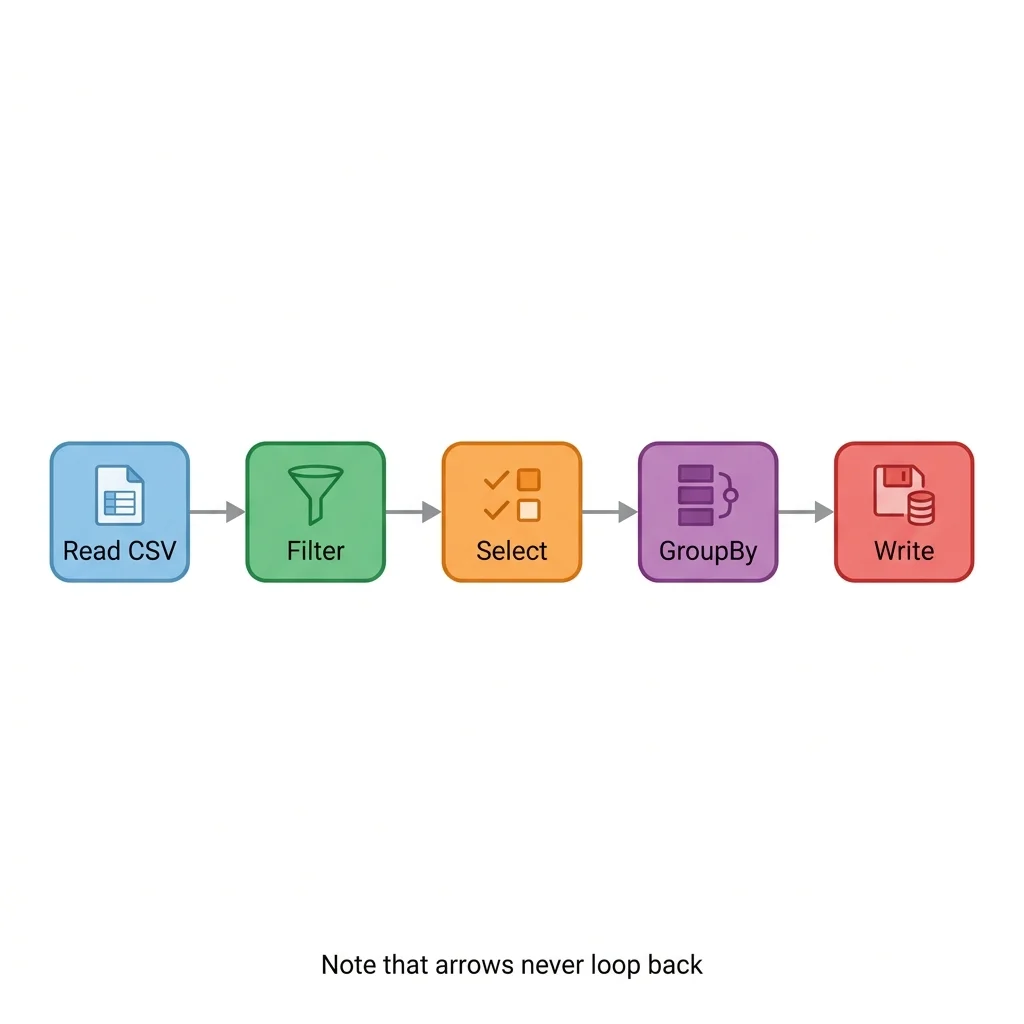
• Directed — the edges have a direction: data flows from source toward result. Read → filter → group → output, never backwards.
• Acyclic — no cycles. The flow never loops back on itself; you can't have step A depend on step B which depends on step A. It's a one-way pipeline from input to output.

So a Spark DAG is simply a one-way flowchart of your whole computation, from reading the source to producing the result. The driver (Module 02) builds this DAG as you chain transformations, and it's this DAG that the driver later slices into stages and tasks when an action fires.

---

From logical plan to physical plan

When an action finally triggers execution, Spark doesn't just run the DAG as-written. It puts your plan through a refinement pipeline, turning what you asked for into the most efficient way to actually do it. At a high level:

1. Logical plan — a representation of what you want, independent of how it'll run. Spark takes your DAG of transformations and forms this logical plan, then optimizes it using rules (reorder, prune, simplify — more below).
2. Physical plan — the optimized logical plan is translated into a concrete how: specific execution strategies (which join algorithm, how to exchange data), ready to run as tasks on executors.

The engine that performs this logical-to-physical refinement is the Catalyst optimizer, and it's important enough to get its own module (08). The point for now is simply: laziness is what makes this optimization possible at all. If Spark ran each transformation eagerly the instant you wrote it, it would have already committed to a way of doing things before it ever saw the next step. By waiting, it gets to see the entire query and rearrange it freely before a single byte is read.

The core payoff, stated plainly: eager execution optimizes one step at a time (locally, blindly). Lazy execution optimizes the whole query at once (globally, with foresight). That's why Spark is lazy.

---

The optimizations laziness unlocks

Abstract claims about "optimization" are unconvincing without examples, so here are the concrete wins — the reasons laziness earns its keep.

Predicate pushdown

This is the classic, most intuitive example. Suppose you read a large table and, several steps later, filter it down to a tiny subset:

# What you WROTE: read everything, do some work, then filter at the end.
df = spark.read.parquet("/data/huge_table")
result = (df
          .select("id", "country", "amount")
          .withColumn("amount_usd", df.amount * 1.1)
          .filter(df.country == "Japan"))   # filter appears LAST
result.show()

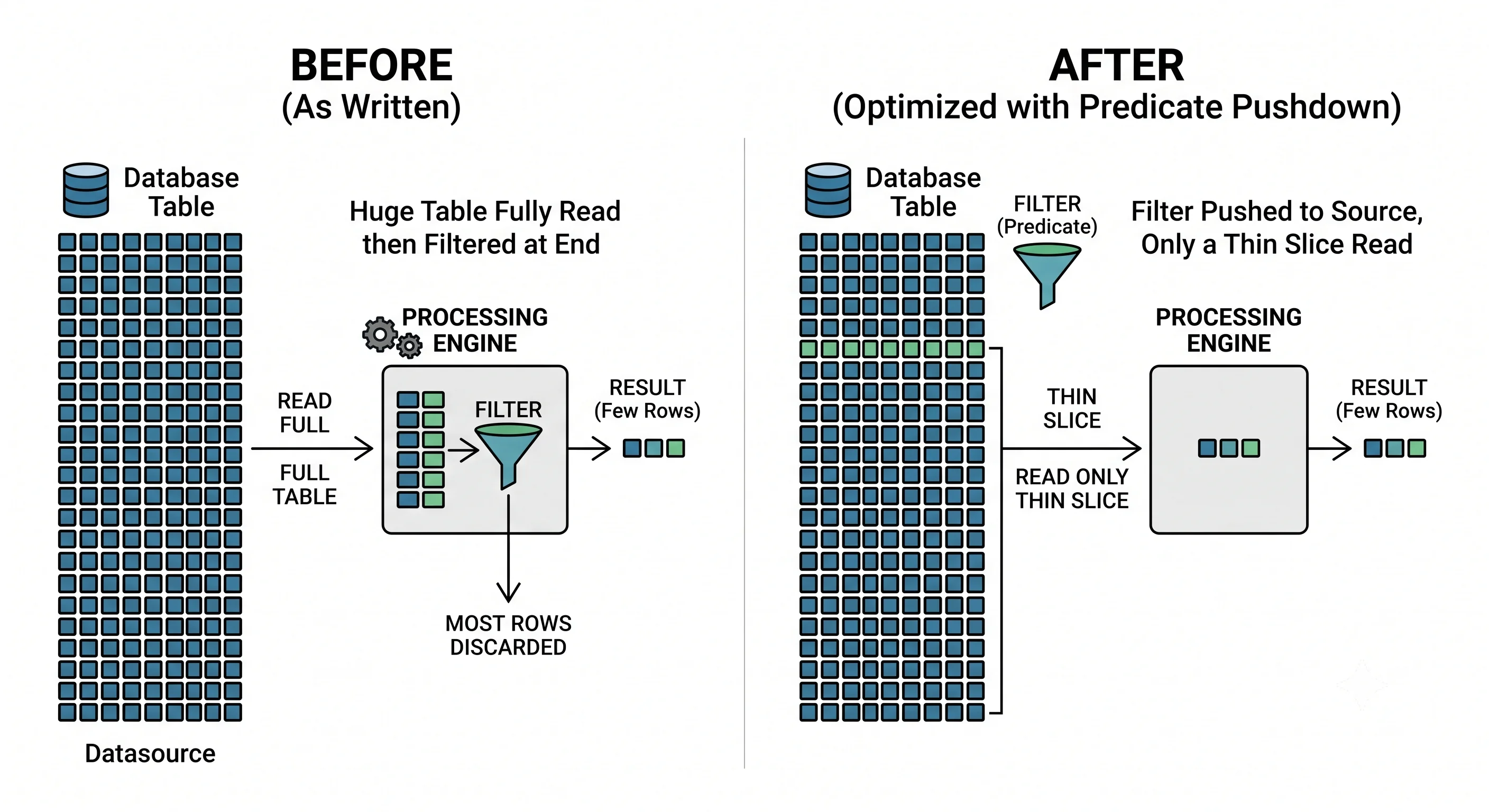
Naively, this reads the entire huge table, transforms every row, and only then throws almost all of it away. A wasteful order. Because Spark saw the whole plan before running it, it can push the filter down to the data source — reading only the country == "Japan" rows in the first place (Parquet can even skip whole files/row-groups). You wrote the filter last; Spark runs it first. Same result, a fraction of the I/O. This is predicate pushdown, and you get it for free precisely because Spark was lazy enough to see the filter before it started reading.

Pipelining of narrow transformations

Recall from Module 05 that consecutive narrow transformations can be pipelined — fused into a single pass over each partition, in memory, without writing intermediate results. Spark can only do this fusion because it sees the chain of narrow operations together in the plan, rather than executing each one as an isolated step.

Other rule-based rewrites

Because it holds the full plan, Spark can also:

• Prune columns it can prove you never use (projection pruning), so it never reads or carries them.
• Combine and simplify operations — folding constants, simplifying boolean expressions, collapsing redundant steps.
• Reorder operations to do cheap, data-reducing work (like filters) as early as possible.

Every one of these depends on the same thing: Spark having the whole query in hand before it commits to running it. Take away laziness and you take away all of it.

---

Seeing it for yourself: explain()

You don't have to take any of this on faith. Spark will show you the plan it intends to run via the .explain() method — an action-like inspection that prints the physical plan (and optionally the logical stages) without processing your data end to end.

result = (spark.read.parquet("/data/huge_table")
          .select("id", "country", "amount")
          .filter("country = 'Japan'"))

# Print the physical plan Spark will execute.
result.explain()

# For the full journey — parsed, analyzed, optimized logical plans, then physical:
result.explain(mode="extended")

When you read the output, look for two revealing things:

• PushedFilters in the scan node — proof that predicate pushdown happened; your filter is being applied at the data source.
• Exchange — this is Spark's word for a shuffle. Every Exchange in the plan marks a wide transformation and a stage boundary (Modules 05 and 07). Counting the Exchange nodes is a fast way to gauge how shuffle-heavy — and therefore how expensive — a query is.

Reading query plans is a genuine superpower for diagnosing slow jobs. You'll see explain() again throughout Part V; for now, just know that the plan is inspectable and that Exchange = shuffle = "here be dragons."

---

A subtle consequence: laziness recomputes

One practical gotcha falls straight out of laziness. Because a DataFrame is just a recorded plan, each action re-runs the whole plan from the beginning. If you call two actions on the same DataFrame, Spark computes it twice:

df = spark.read.parquet("/data/huge_table").filter("country = 'Japan'")

df.count()   # Job 1: reads and filters the whole source
df.show()    # Job 2: reads and filters the whole source AGAIN

Spark doesn't remember the result of the first action unless you tell it to. When you're going to reuse a DataFrame across multiple actions, that's exactly when you cache it — the subject of Module 15. For now, file away: laziness is powerful, but it means "compute" is tied to actions, and repeated actions mean repeated work.

---

Key takeaways

• Lazy evaluation: Spark records transformations and defers all computation until an action forces it — the opposite of eager, line-by-line execution.
• While waiting, Spark builds lineage and a DAG (Directed Acyclic Graph) — a one-way, no-loops flowchart of the whole computation from source to result.
• On an action, Spark refines a logical plan (the what) into an optimized physical plan (the how) via the Catalyst optimizer (Module 08). Laziness is what makes whole-query optimization possible.
• Concrete wins include predicate pushdown (run filters at the source, reading far less data), pipelining of narrow transformations, projection pruning, and expression simplification/reordering.
• Inspect any plan with .explain(); look for PushedFilters (pushdown worked) and Exchange (a shuffle / stage boundary).
• Because a DataFrame is just a plan, each action recomputes it from scratch — the motivation for caching (Module 15).

---

Check your understanding

1. Explain, using the GPS analogy, why optimizing the whole query at once beats optimizing one transformation at a time.
2. You write a .filter() as the very last step of a long query on a huge table. What does predicate pushdown do with it, and why is Spark's laziness a prerequisite?
3. You run df.count() and then df.show() on the same uncached DataFrame built from an expensive read. How many times is the source read, and what would you change to fix it?

---

Up next

The Shuffle — The Shuffle. We've now named the shuffle repeatedly as "the most expensive operation" and seen it appear as Exchange in query plans. Next we finally open it up: what physically happens during a shuffle's map/shuffle/sort/reduce phases, which operations cause it, and the concrete techniques to reduce it.