SparkSession Getting Started

Part IV — Writing PySpark · Module 9 of 18 Prerequisites: Spark Architecture (the driver & SparkSession), Partitions & Parallelism You will learn: how to create and configure a SparkSession (the one entry point to everything), how to read data into a DataFrame, and — critically — why you should almost always supply an explicit schema instead of letting Spark guess.

---

Part IV: from theory to typing

You've spent eight modules building a mental model of how Spark thinks. Now we start writing it. Part IV is hands-on PySpark, and everything begins in the same place every Spark program does: the SparkSession.

---

The SparkSession: your single doorway

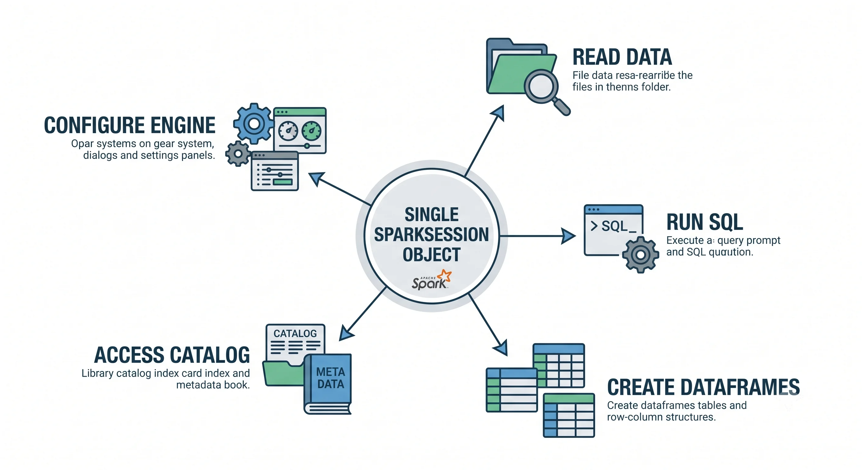
We met the SparkSession in Module 02 as the object the driver holds. Here's the practical framing: the SparkSession is your unified entry point to every Spark capability. Reading data, running SQL, creating DataFrames, reaching catalog metadata, configuring the engine — all of it flows through this one object.

Since Spark 2.0, it subsumes the older, separate context objects — SparkContext, SQLContext, HiveContext, StreamingContext — that earlier versions forced you to juggle. One object now opens every door.

Analogy — the master key. Older Spark was like a building where you carried a separate key for each room: one for SQL, one for streaming, one for core operations. The SparkSession is a single master key that opens every room. You carry one thing, and it works everywhere.

Creating one with the builder

You construct a SparkSession with the builder pattern — a readable chain of configuration calls ending in getOrCreate():

from pyspark.sql import SparkSession

spark = (SparkSession
         .builder
         .appName("GettingStartedApp")                      # name shown in the Spark UI
         .config("spark.sql.shuffle.partitions", 8)         # tune shuffle partitions (Module 07)
         .getOrCreate())                                     # reuse or create the session

Two pieces deserve a note:

• .appName(...) sets the name you'll see in the Spark UI — invaluable when hunting down a job among many (Module 17's debugging).
• .getOrCreate() does exactly what it says: if a SparkSession already exists (common in notebooks and shells, where one is often pre-created for you), it reuses it; otherwise it creates a new one. This prevents you from accidentally spinning up multiple competing sessions.

Note on managed environments. In Databricks notebooks, spark-shell, pyspark, and many hosted platforms, a SparkSession named spark is already created for you. You can just use spark directly. You mainly call the builder yourself in standalone scripts submitted via spark-submit.

Configuring the session

You can set configuration at build time (as above) or afterward on a live session:

# Read or change a config on an existing session
spark.conf.set("spark.sql.shuffle.partitions", 16)
print(spark.conf.get("spark.sql.shuffle.partitions"))

# Useful bits of info
print(spark.version)          # Spark version

Most tuning knobs from Parts III and V (spark.sql.shuffle.partitions, spark.sql.files.maxPartitionBytes, broadcast thresholds, Adaptive Query Execution) are set exactly this way.

---

Reading data into a DataFrame

With a session in hand, you load data through spark.read, choosing a format and pointing at a source:

# General shape: spark.read.format(...).option(...).load(path)
df = (spark.read
      .format("csv")
      .option("header", "true")
      .load("/data/flights/departuredelays.csv"))

# Common formats: "csv", "json", "parquet", "orc". Parquet is the default and preferred.
parquet_df = spark.read.parquet("/data/flights/summary.parquet")

A quick but important aside: prefer columnar formats like Parquet for anything beyond quick experiments. Parquet stores data by column, carries the schema with the data, and supports the predicate pushdown and column pruning Catalyst loves (Modules 06, 08). CSV and JSON are convenient for input but slow and schema-less by comparison.

---

The schema decision: don't make Spark guess

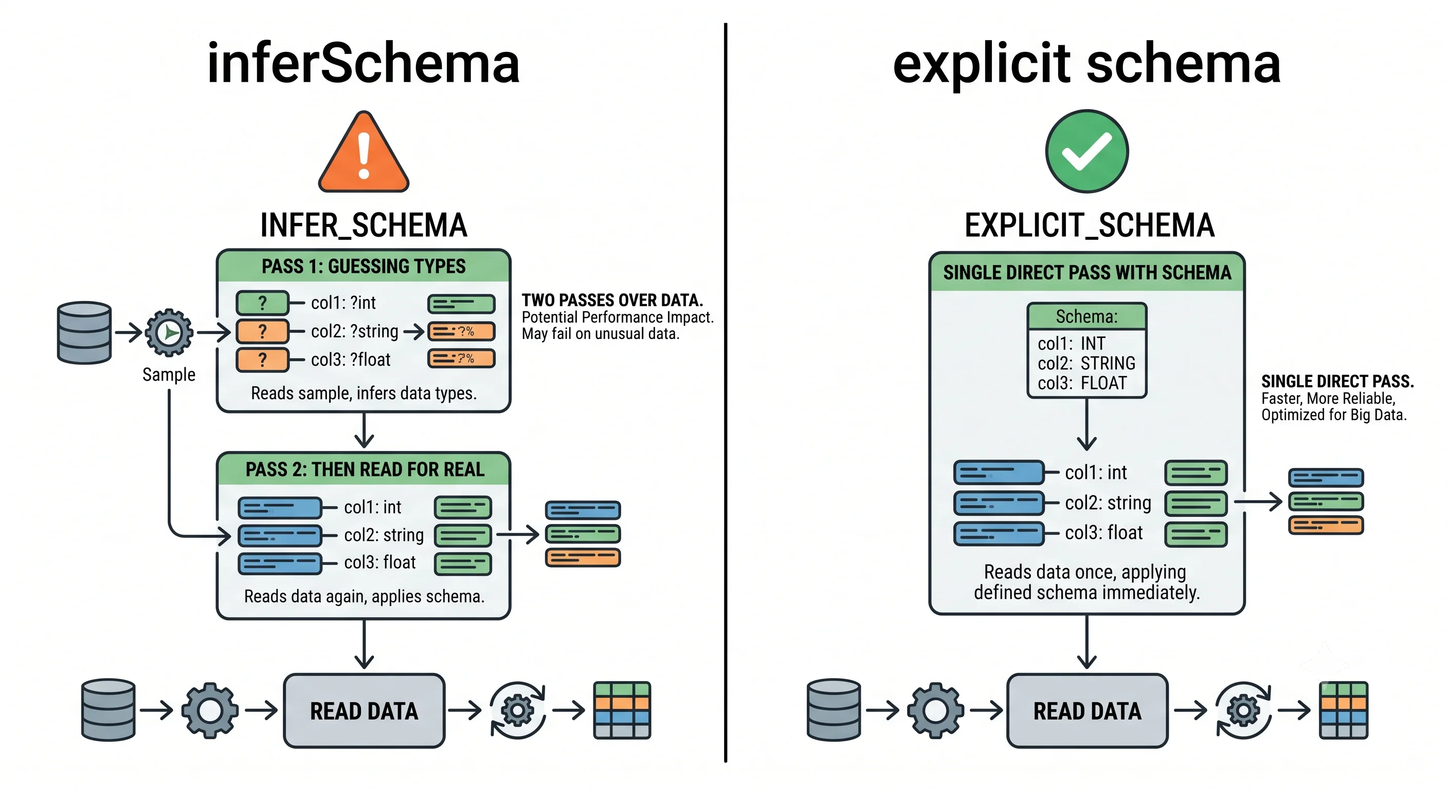
Here is the single most important habit in this module. When you read data, Spark needs to know the schema — the column names and their types. You have two options, and the difference matters for both correctness and performance.

Option A (tempting, but costly): schema inference

You can ask Spark to figure out the schema itself with inferSchema:

# Convenient... but Spark must READ THROUGH the data first just to guess the types.
df = (spark.read
      .option("header", "true")
      .option("inferSchema", "true")   # <-- the costly part
      .csv("/data/flights/departuredelays.csv"))

This works, and it's fine for a quick look at a small file. But inferSchema forces Spark to make an extra pass over the data just to sample and deduce types before your real query even begins. On a large dataset that's a significant, wasted read. Worse, inference can guess wrong — reading a ZIP code as an integer and stripping leading zeros, or misjudging a column that's mostly numbers but occasionally text.

Option B (recommended): an explicit schema

Tell Spark the schema up front. It skips the inference pass entirely — reading immediately and correctly. There are two clean ways to express it.

B1 — a DDL string (concise and very readable):

# Define the schema as a simple DDL-style string.
schema_ddl = "date STRING, delay INT, distance INT, origin STRING, destination STRING"

df = (spark.read
      .format("csv")
      .option("header", "true")
      .schema(schema_ddl)               # explicit — no inference pass, no wrong guesses
      .load("/data/flights/departuredelays.csv"))

B2 — a programmatic StructType (verbose, but powerful for building schemas in code):

from pyspark.sql.types import StructType, StructField, StringType, IntegerType

schema_struct = StructType([
    StructField("date",        StringType(),  True),   # True = nullable
    StructField("delay",       IntegerType(), True),
    StructField("distance",    IntegerType(), True),
    StructField("origin",      StringType(),  True),
    StructField("destination", StringType(),  True),
])

df = (spark.read
      .format("csv")
      .option("header", "true")
      .schema(schema_struct)
      .load("/data/flights/departuredelays.csv"))

Both produce the identical result. Use the DDL string for readability in everyday code; use StructType when you need to construct or manipulate schemas programmatically (e.g., generating them dynamically).

The rule to internalize: in any serious pipeline, always define the schema explicitly. You avoid the wasteful inference read, you eliminate silent type-guessing bugs, and your code documents exactly what it expects. Reserve inferSchema for throwaway exploration.

---

Inspecting what you loaded

Once data is in a DataFrame, a few everyday methods confirm you got what you expected:

df.printSchema()      # show column names and types as a tree
df.show(5)            # display the first 5 rows (an ACTION — triggers execution)
print(df.count())     # number of rows (also an action)
print(df.columns)     # list of column names

Remember from Module 05 that show() and count() are actions — they actually run the plan — whereas simply reading and describing the DataFrame builds the plan lazily. printSchema() and columns, by contrast, only inspect metadata and don't process your data.

---

A bridge to Spark SQL: temporary views

One more capability the SparkSession unlocks, which we'll build on in Module 11: you can register any DataFrame as a temporary view and then query it with plain SQL.

# Register the DataFrame as a queryable SQL view (lives for this session).
df.createOrReplaceTempView("flights")

# Now query it with SQL through the same SparkSession.
top = spark.sql("""
    SELECT origin, COUNT(*) AS n
    FROM flights
    GROUP BY origin
    ORDER BY n DESC
    LIMIT 5
""")
top.show()

This is a preview of a theme from Module 04 and 08: the SQL string and the equivalent DataFrame code compile to the same Catalyst plan, so you can freely mix whichever is clearer for a given task. Module 11 explores this interoperability in full.

---

Key takeaways

• The SparkSession is your single unified entry point to all of Spark; since 2.0 it subsumes the old SparkContext/SQLContext/HiveContext/StreamingContext.
• Create it with the builder pattern ending in .getOrCreate() (which reuses an existing session or makes a new one). In notebooks/shells a spark session is usually pre-created.
• Set configuration at build time via .config(...) or later via spark.conf.set(...).
• Read data with spark.read.format(...).option(...).load(...); prefer Parquet for real workloads (columnar, carries its schema, pushdown-friendly).
• Always define an explicit schema for serious pipelines — via a DDL string (readable) or a StructType (programmatic). It avoids the wasteful inferSchema extra pass and silent type-guessing bugs; reserve inference for quick exploration.
• Inspect with printSchema(), show(), count(), columns — remembering show()/count() are actions.
• Register a DataFrame as a temporary view to query it with SQL (same Catalyst plan as the DataFrame API — full story in Module 11).

---

Check your understanding

1. What does .getOrCreate() do, and why is it safer than always constructing a fresh SparkSession?
2. Give two concrete reasons to supply an explicit schema instead of using inferSchema on a large production dataset.
3. Which of these actually process your data when called: printSchema(), show(5), count(), columns? Explain using the transformation/action distinction.

---

Up next

DataFrame Operations — DataFrame Operations. With a session created and data loaded, we get to the daily toolkit: selecting, filtering, grouping, aggregating, and adding/renaming/dropping columns — the operations you'll use in almost every PySpark job.