Time-Series Databases

In a Nutshell

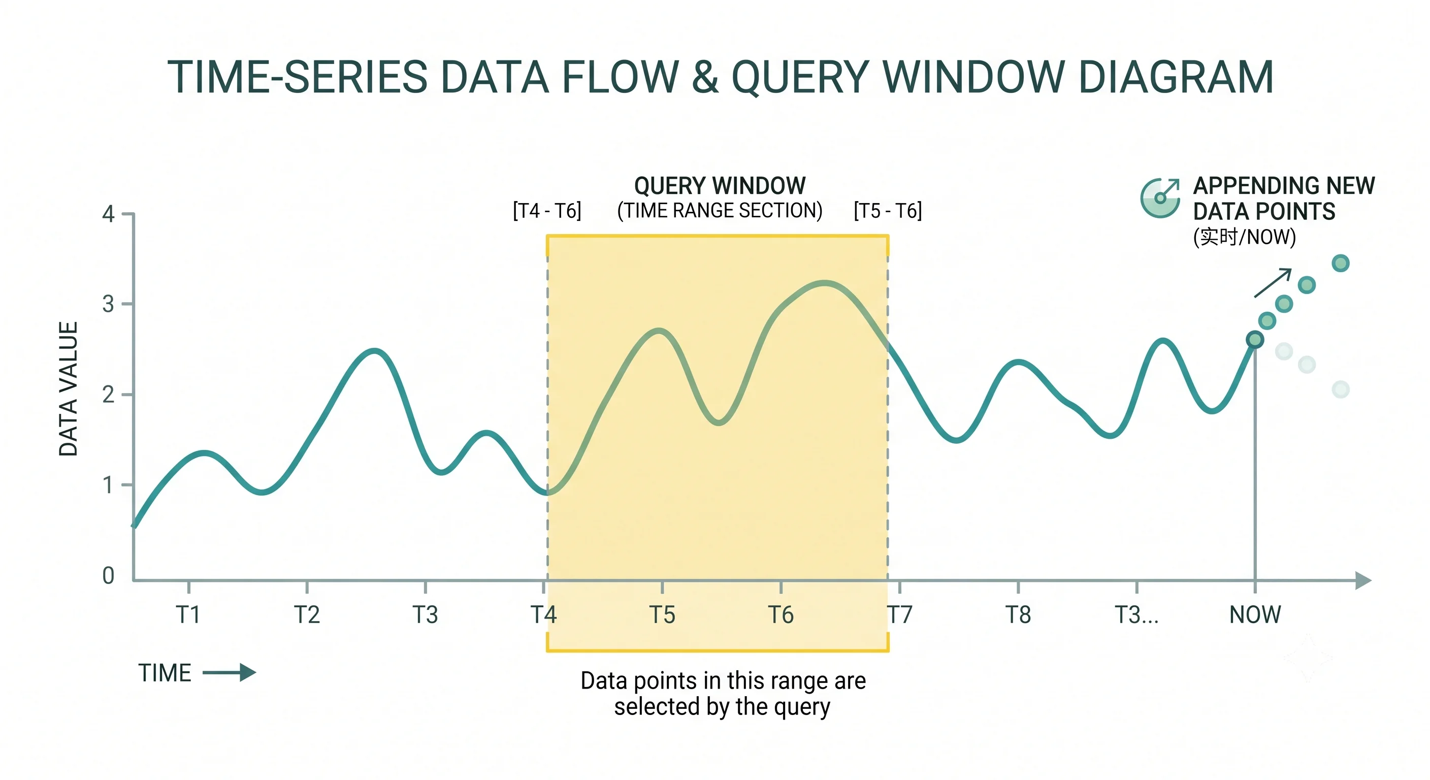
A time-series database (TSDB) is optimized for append-only, time-stamped data — metrics, sensor readings, stock prices, logs, and monitoring data. Every write is a new data point; updates and deletes are rare. The queries are almost always: "What happened between time A and time B?" and "What's the average/max/min over the last hour?" TSDBs exploit this narrow access pattern to achieve extreme compression (10–50× vs general-purpose databases) and fast range queries. If your data has a timestamp and you mostly query by time range, a TSDB will significantly outperform a general-purpose database.

How It Actually Works

What Makes TSDBs Special

Feature	How TSDBs Optimize
Compression	Delta-of-delta, Gorilla encoding — consecutive timestamps are very similar, so only differences are stored
Write path	Append-only (LSM-tree or WAL) — no random I/O, sequential writes only
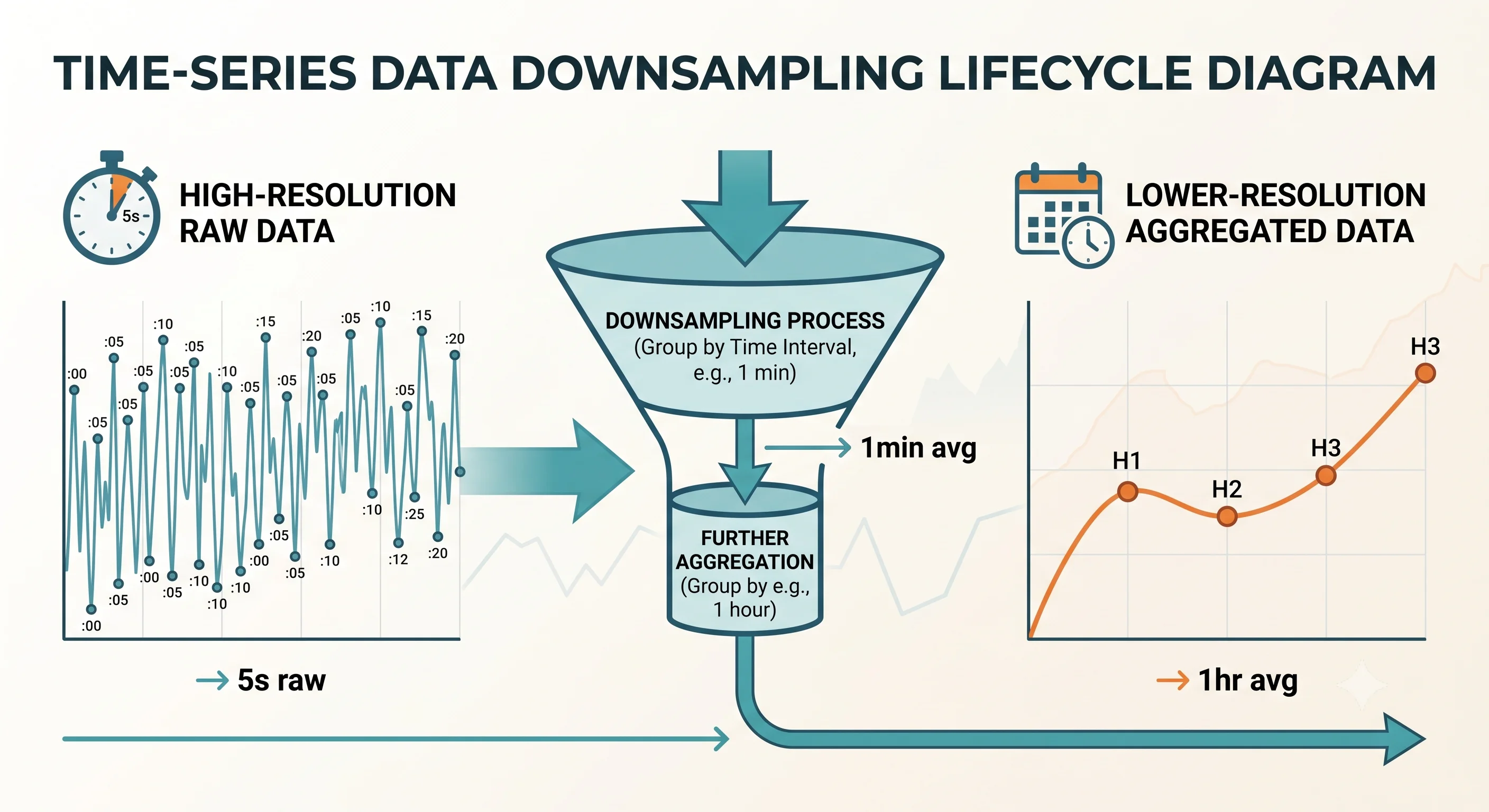
Retention policies	Automatic downsampling (5-second data → 1-minute averages after 30 days → hourly after 1 year)
Aggregation	Built-in functions: rollups, moving averages, percentiles over time windows
Partitioning	Data is automatically partitioned by time range (e.g., daily chunks)

The Major Players

Database	Language	Best For	Used By
Prometheus	PromQL	Pull-based monitoring, Kubernetes metrics	Cloud-native monitoring
InfluxDB	InfluxQL / Flux	IoT, application metrics, general purpose TSDB	Telegraf + Grafana stack
TimescaleDB	SQL (PostgreSQL extension)	Teams that want TSDB performance with SQL familiarity	PostgreSQL users needing time-series
ClickHouse	SQL	Analytics on time-series and event data at scale	Observability platforms, product analytics
QuestDB	SQL	Ultra-low latency ingestion	Financial data, real-time analytics

Prometheus + Grafana (The Monitoring Stack)

The most common time-series setup for infrastructure monitoring:

┌──────────┐    scrape    ┌────────────┐    query     ┌──────────┐
│  App +   │◀─────────────│ Prometheus │◀─────────────│ Grafana  │
│ /metrics │   (pull)     │  (TSDB)    │  (PromQL)    │(dashboard)│
│ endpoint │              └──────┬─────┘              └──────────┘
└──────────┘                     │
                           ┌─────▼──────┐
                           │ Alertmanager│──▶ Slack, PagerDuty
                           └────────────┘

When to Choose a TSDB

✅ Use when:

• Data is append-only with timestamps (metrics, sensors, logs)
• Primary queries are time-range based ("last 24 hours," "last 7 days")
• You need automatic downsampling and retention policies
• Compression ratio matters (storing months/years of data cheaply)

❌ Don't use when:

• Data needs updates or deletes regularly (use SQL)
• Queries are not time-based (use SQL or NoSQL)
• Data has complex relationships (use SQL or graph)
• You need transactional guarantees (use SQL)

Seeing It in Action

Scenario: Application performance monitoring

# PromQL examples

# Average request latency over 5 minutes, by endpoint
rate(http_request_duration_seconds_sum[5m])
  / rate(http_request_duration_seconds_count[5m])

# 99th percentile latency
histogram_quantile(0.99, rate(http_request_duration_seconds_bucket[5m]))

# Error rate (5xx responses / total responses)
sum(rate(http_responses_total{status=~"5.."}[5m]))
  / sum(rate(http_responses_total[5m]))

# Alert: fire if error rate > 1% for 5 minutes
alert: HighErrorRate
expr: sum(rate(http_responses_total{status=~"5.."}[5m]))
      / sum(rate(http_responses_total[5m])) > 0.01
for: 5m

Why a TSDB is right here:

• High cardinality — Thousands of metrics × labels (endpoint, method, status code) = millions of time-series
• Compression — Raw metrics for 10K containers would consume TB in SQL; Prometheus stores it in GB
• Built-in functions — rate(), histogram_quantile(), increase() — purpose-built for monitoring
• Retention — Keep 15 days of raw data, downsample to hourly for long-term storage

Interview Questions

1. Q: When would you choose a time-series database over PostgreSQL for metrics storage? Hint: When you have millions of time-series, need extreme compression, require built-in downsampling, and all queries are time-range based. PostgreSQL can handle small-scale time-series with TimescaleDB, but at monitoring scale (millions of series, weeks of data), a dedicated TSDB is dramatically more efficient.

2. Q: What is downsampling, and why is it important for time-series data? Hint: Reducing resolution over time: keep 1-second data for 24 hours, aggregate to 1-minute averages for 30 days, hourly for a year. Without downsampling, storage grows linearly and queries over long ranges become slow. Downsampling trades precision for storage efficiency — you don't need 1-second granularity for last year's data.

3. Q: Explain the difference between Prometheus (pull-based) and InfluxDB (push-based) monitoring. Hint: Prometheus scrapes (pulls) metrics from targets at regular intervals — simpler to operate, targets don't need to know about Prometheus, but requires service discovery. InfluxDB receives (push) metrics from agents — better for ephemeral targets (serverless, short-lived containers), but agents need to be configured with the InfluxDB endpoint. Prometheus is the Kubernetes standard.

4. Q: How would you handle high-cardinality time-series data (e.g., per-user metrics)? Hint: High cardinality (unique label combinations) explodes the number of time-series and is the #1 cause of TSDB performance problems. Solutions: avoid per-user labels in metrics (use logging/tracing instead), pre-aggregate where possible, use databases designed for high cardinality (ClickHouse, QuestDB), and set cardinality limits.

5. Q: You need to store IoT sensor data for 5 years with per-second resolution. How do you manage the storage? Hint: Tiered retention: keep raw (1-second) data for 7–30 days in the TSDB. Downsample to 1-minute averages for 90 days, 1-hour averages for 1 year, and daily aggregates for 5 years. Move cold data to object storage (S3/Parquet) for long-term archival. Math: 1M sensors × 1 reading/sec × 100 bytes = 8.6 TB/day raw — downsampling reduces this by 60× (1-minute) to 3600× (1-hour).

References

• Prometheus Documentation — official docs with PromQL reference
• InfluxDB Documentation — official InfluxDB guides
• TimescaleDB Documentation — PostgreSQL extension for time-series

Dive Deeper

• Gorilla: A Fast, Scalable, In-Memory Time-Series Database — Facebook's time-series compression paper
• ClickHouse for Time-Series — using ClickHouse for analytics on time-series data
• Thanos / Cortex — long-term storage and multi-cluster federation for Prometheus