Wide-Column Stores

In a Nutshell

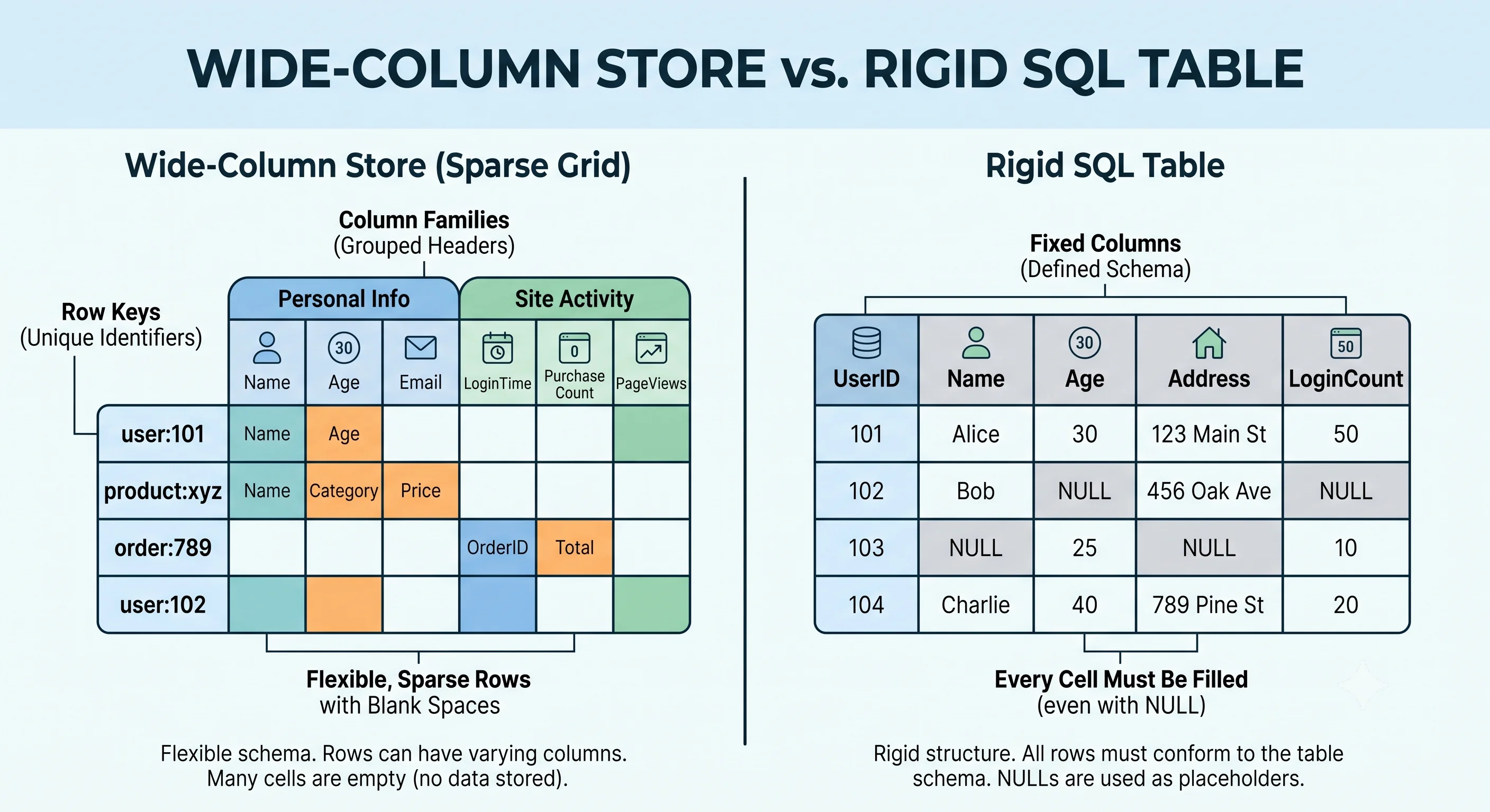
Wide-column stores are optimized for massive write throughput and time-ordered data. Unlike a relational table where every row has the same fixed columns, each row in a wide-column store can have different columns, and columns are grouped into column families. You model the table around the query you intend to run — not around the data itself. This makes them ideal for IoT sensor data, activity logs, messaging, and any workload with billions of writes per day. Cassandra, HBase, and ScyllaDB are the key players.

How It Actually Works

Data Model

Row Key         │ Column Family: profile          │ Column Family: activity
────────────────┼─────────────────────────────────┼──────────────────────────
user:alice      │ name: "Alice"                   │ 2024-01-15: "login"
                │ email: "alice@example.com"       │ 2024-01-15: "post_created"
                │ city: "SF"                       │ 2024-01-16: "login"
────────────────┼─────────────────────────────────┼──────────────────────────
user:bob        │ name: "Bob"                     │ 2024-01-16: "login"
                │ email: "bob@example.com"         │
                │                                  │ (sparse — no city column)

Key concepts:

• Row key (partition key) — determines which node stores the row. This is the most important design decision.
• Column families — groups of related columns, defined at schema creation. Each family can have different storage settings.
• Columns — can be added dynamically per row. No ALTER TABLE needed.
• Sorted by column name — within a row, columns are sorted, enabling range queries within a row.

Cassandra — The Most Popular Wide-Column Store

Feature	Description
Architecture	Peer-to-peer ring (no master node) — any node can accept reads/writes
Consistency	Tunable: ONE, QUORUM, ALL (per query)
Partition key	Determines data placement — choose for even distribution
Clustering key	Determines sort order within a partition
Compaction	LSM-tree based — writes go to memtable, flush to SSTables, compact periodically
Replication	Configurable replication factor (typically 3) across datacenters

The Critical Rule: Model the Query, Not the Data

In Cassandra, you cannot do:

• Joins
• Ad-hoc queries on non-key columns (without secondary indexes, which are slow)
• Aggregations across partitions efficiently

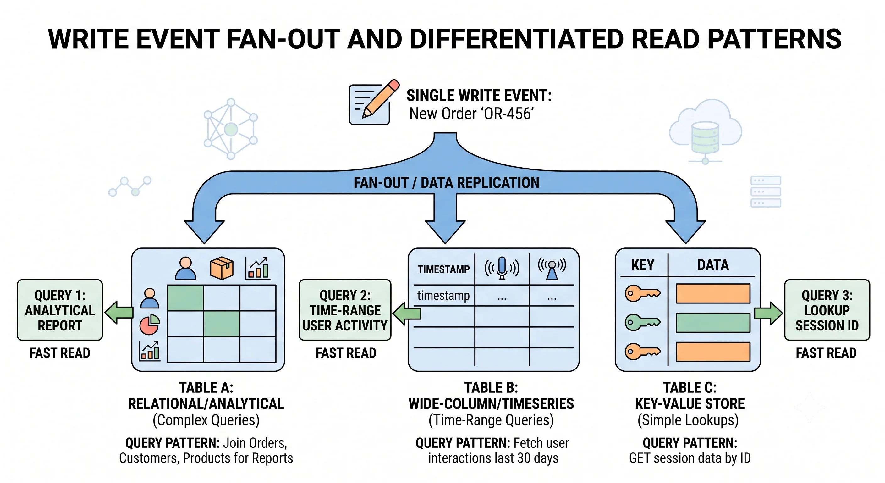
Instead, you create a separate table for each query pattern:

-- Query 1: Get all messages in a conversation, sorted by time
CREATE TABLE messages_by_conversation (
    conversation_id UUID,
    sent_at         TIMESTAMP,
    sender_id       UUID,
    content         TEXT,
    PRIMARY KEY (conversation_id, sent_at)
) WITH CLUSTERING ORDER BY (sent_at DESC);

-- Query 2: Get all messages sent by a user
CREATE TABLE messages_by_user (
    sender_id       UUID,
    sent_at         TIMESTAMP,
    conversation_id UUID,
    content         TEXT,
    PRIMARY KEY (sender_id, sent_at)
) WITH CLUSTERING ORDER BY (sent_at DESC);

Same data, two tables. You write to both on every message send. This is write amplification — the cost of read optimization.

When to Choose Wide-Column

✅ Use when:

• Write throughput is extremely high (millions/second)
• Data is time-ordered or append-heavy (logs, metrics, IoT)
• Query patterns are known in advance and limited
• You need multi-datacenter replication with tunable consistency
• Data volume is in the terabytes to petabytes

❌ Don't use when:

• You need ad-hoc queries (use SQL)
• Data has complex relationships (use SQL or graph DB)
• You need strong consistency for every operation (use SQL or NewSQL)
• Query patterns will change frequently (each change may require a new table)

Seeing It in Action

Scenario: IoT sensor data platform (1M devices, 1 reading/second each)

-- Table designed for: "Get readings for device X in a time range"
CREATE TABLE sensor_readings (
    device_id   UUID,
    bucket      TEXT,           -- e.g., '2024-01-15' (prevents unbounded partitions)
    recorded_at TIMESTAMP,
    temperature FLOAT,
    humidity    FLOAT,
    pressure    FLOAT,
    PRIMARY KEY ((device_id, bucket), recorded_at)
) WITH CLUSTERING ORDER BY (recorded_at DESC);

Write volume math:

• 1M devices × 1 reading/sec = 1M writes/second
• Each reading ~100 bytes → 100 MB/second → 8.6 TB/day
• This is exactly what Cassandra is built for

Key design decisions:

• Partition key: (device_id, bucket) — distributes data across nodes and prevents unbounded partition growth
• Bucketing by day: Without it, a device running for a year would have 31M rows in one partition (too large). Daily buckets keep partitions under ~100K rows.
• Clustering key: recorded_at DESC — most recent readings first (most common query pattern)

Interview Questions

1. Q: Why can't you do ad-hoc queries efficiently in Cassandra? Hint: Cassandra distributes data by partition key using consistent hashing. A query that doesn't include the partition key requires a full cluster scan — contacting every node. The data model assumes you know your query patterns at design time and build tables to serve each one.

2. Q: What happens if you choose a bad partition key in Cassandra? Hint: Hot partition — one node gets disproportionate traffic. Example: partitioning sensor data by country when 80% of devices are in one country. The fix: use a high-cardinality key (device_id) or composite key. Monitor partition sizes and heat maps.

3. Q: How does Cassandra's tunable consistency work? When would you use QUORUM vs ONE? Hint: ONE: write/read acknowledged by 1 replica — fastest, but might read stale data. QUORUM: majority must agree — strong consistency (if write QUORUM + read QUORUM > replication factor). ALL: every replica — slowest, most consistent, least available. Use QUORUM for important data, ONE for metrics/logs where staleness is acceptable.

4. Q: Explain write amplification in wide-column stores. Is it a problem? Hint: Same data written to multiple tables (one per query pattern). A chat message might be written to messages_by_conversation, messages_by_user, and messages_by_date — 3× write amplification. It's acceptable because: Cassandra writes are extremely fast (append-only, LSM-tree), and reads are critical-path while writes are often async.

5. Q: How would you choose between Cassandra and a time-series database (InfluxDB) for IoT data? Hint: Cassandra: when you need multi-datacenter replication, tunable consistency, and data isn't purely time-series (e.g., you also query by device metadata). InfluxDB: when data is purely time-series metrics, you need built-in downsampling/aggregation, and single-region is sufficient. InfluxDB has better compression for time-series but less flexibility.

References

• Apache Cassandra Documentation — official docs with data modeling guides
• Designing Data-Intensive Applications by Martin Kleppmann — Chapter 2 on column-family stores
• Cassandra Data Modeling Best Practices — DataStax guide

Dive Deeper

• Cassandra: The Definitive Guide by Jeff Carpenter & Eben Hewitt — comprehensive Cassandra reference
• ScyllaDB — A Better Cassandra? — C++ reimplementation with 10× throughput claims
• Discord's Cassandra to ScyllaDB Migration — real-world case study of wide-column at scale