Indexing

In a Nutshell

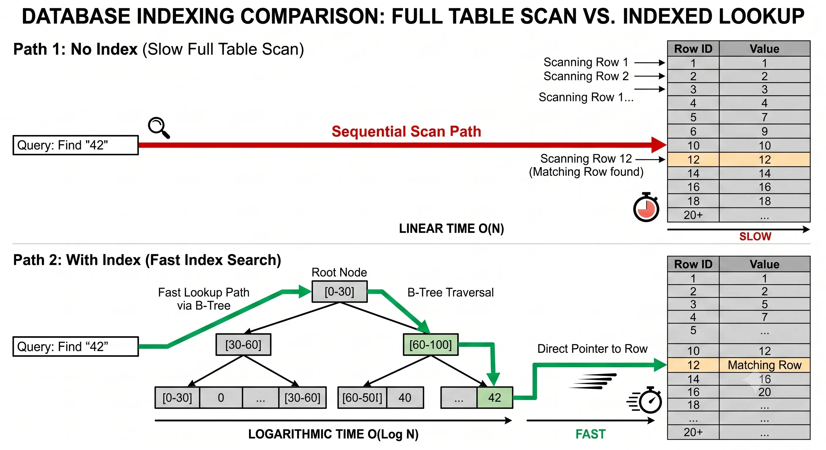
Without an index, every query is a full table scan — the database reads every row to find what you need. With the right index, the same query touches only the relevant rows. This is the difference between O(n) and O(log n) — and at scale, the difference between a 50ms query and a 5-second query. Indexing is the single most impactful performance optimization available in any database. But indexes aren't free: every index speeds up reads and slows down writes (because the index must be updated on every insert/update/delete).

How It Actually Works

B-Tree Index (The Default)

The most common index structure. It's a balanced tree where each node contains sorted keys and pointers to child nodes (or data rows).

                    [50]
                   /    \
              [20, 35]   [70, 85]
             / |  \     / |  \
           [10] [25] [40] [60] [75] [90]
            ↓    ↓    ↓    ↓    ↓    ↓
          rows  rows rows rows rows rows

• Lookup: O(log n) — traverse from root to leaf
• Range query: O(log n + k) — find the start, then scan leaves sequentially
• Insert/Delete: O(log n) — find the position, insert/remove, rebalance

Index Types

Type	Structure	Best For	Example
B-Tree	Balanced tree	Equality + range queries (default)	WHERE age > 25 AND age < 35
Hash	Hash table	Exact equality only	WHERE email = 'alice@example.com'
Composite	B-tree on multiple columns	Multi-column queries	WHERE city = 'SF' AND age > 25
Covering	Includes all queried columns	Avoiding table lookup	Index includes (city, name, email)
Partial	Index only rows matching a condition	Filtering out common values	WHERE status = 'active' (skip inactive rows)
Full-text	Inverted index	Text search	WHERE body @@ 'database performance'
GIN	Generalized Inverted Index	JSONB, arrays, full-text	WHERE tags @> '{"urgent"}'
GiST	Generalized Search Tree	Geospatial, range types	WHERE location <-> point(37.7, -122.4) < 1000

Composite Index and the Leftmost Prefix Rule

A composite index on (city, age, name) can serve queries on:

• ✅ WHERE city = 'SF' (first column)
• ✅ WHERE city = 'SF' AND age > 25 (first two columns)
• ✅ WHERE city = 'SF' AND age > 25 AND name = 'Alice' (all three)
• ❌ WHERE age > 25 (skips the first column — can't use this index)
• ❌ WHERE name = 'Alice' (skips the first two columns)

Rule: A composite index is used from left to right. If you skip a column, everything after it is unusable.

The Write Cost of Indexes

Operation	Without Index	With 1 Index	With 5 Indexes
INSERT	Write 1 row	Write 1 row + update 1 index	Write 1 row + update 5 indexes
UPDATE (indexed column)	Update 1 row	Update 1 row + update 1 index	Update 1 row + update affected indexes
Disk space	Data only	Data + index (~10–30% overhead per index)	Data + 5× index overhead

Rule of thumb: Index columns you query frequently. Don't index columns that are rarely queried or have very low cardinality (e.g., a boolean is_active column with only 2 values).

EXPLAIN — Your Best Friend

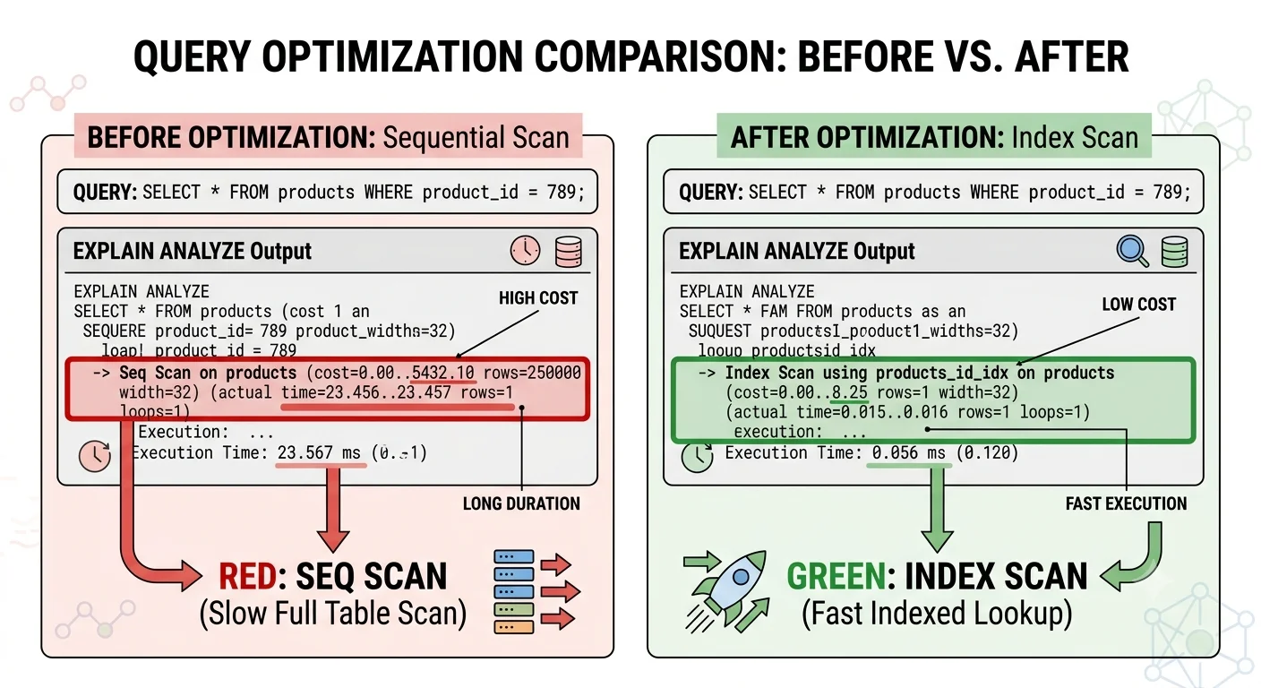
EXPLAIN ANALYZE SELECT * FROM users WHERE email = 'alice@example.com';

-- Without index:
-- Seq Scan on users  (cost=0.00..1250.00 rows=1 width=100) (actual time=15.2ms)
--   Filter: (email = 'alice@example.com')
--   Rows Removed by Filter: 99999

-- With index on email:
-- Index Scan using idx_users_email on users  (cost=0.42..8.44 rows=1 width=100) (actual time=0.03ms)
--   Index Cond: (email = 'alice@example.com')

From 15.2ms (scanning 100K rows) to 0.03ms (direct lookup) — 500× faster.

Seeing It in Action

Scenario: Optimizing queries for an e-commerce product search

-- The table
CREATE TABLE products (
    id          BIGSERIAL PRIMARY KEY,
    name        VARCHAR(200),
    category    VARCHAR(50),
    price       DECIMAL(10,2),
    rating      DECIMAL(3,2),
    in_stock    BOOLEAN DEFAULT true,
    created_at  TIMESTAMP DEFAULT NOW()
);
-- 10 million rows

-- Query 1: Search by category + price range (most common)
-- BEFORE: Seq Scan — 3.2 seconds
SELECT * FROM products WHERE category = 'Electronics' AND price BETWEEN 50 AND 200;

-- FIX: Composite index (leftmost prefix rule satisfied)
CREATE INDEX idx_products_cat_price ON products(category, price);
-- AFTER: Index Scan — 12ms

-- Query 2: Sort by rating within a category
-- BEFORE: Sort + Seq Scan — 4.1 seconds
SELECT * FROM products WHERE category = 'Electronics' ORDER BY rating DESC LIMIT 20;

-- FIX: Composite index with sort direction
CREATE INDEX idx_products_cat_rating ON products(category, rating DESC);
-- AFTER: Index Scan — 0.8ms

-- Query 3: Full-text search on product name
-- BEFORE: Sequential LIKE scan — 8.5 seconds
SELECT * FROM products WHERE name ILIKE '%wireless headphone%';

-- FIX: GIN index with tsvector
CREATE INDEX idx_products_name_fts ON products USING GIN (to_tsvector('english', name));
SELECT * FROM products WHERE to_tsvector('english', name) @@ to_tsquery('wireless & headphone');
-- AFTER: Bitmap Index Scan — 5ms

Interview Questions

1. Q: What's the difference between a B-tree index and a hash index? When would you use each? Hint: B-tree: supports equality AND range queries (=, <, >, BETWEEN), sorted order. Hash: supports only exact equality (=), slightly faster for exact lookups but can't do ranges. Default to B-tree unless you have a very specific equality-only workload.

2. Q: You have a query WHERE status = 'active' AND created_at > '2024-01-01'. What index do you create? Hint: Composite index: (status, created_at). Status first (equality) then created_at (range). Or a partial index: CREATE INDEX ... ON orders(created_at) WHERE status = 'active' — smaller index, faster lookups, but only usable when the WHERE clause matches.

3. Q: Your table has 10 indexes and writes are slow. What do you do? Hint: Audit index usage: pg_stat_user_indexes shows which indexes are actually used. Drop unused indexes. Consolidate overlapping indexes (an index on (a, b) covers queries on a). Consider if some indexes can be partial. Batch writes if possible to amortize index update cost.

4. Q: Why might adding an index make a query slower? Hint: If the query returns a large percentage of the table (e.g., WHERE in_stock = true and 95% of products are in stock), a sequential scan is faster than an index scan + random I/O for each row. The query planner accounts for this — if selectivity is low, it ignores the index. Also, more indexes mean more memory pressure on the buffer pool.

5. Q: How do you index a JSONB column in PostgreSQL? Hint: GIN index: CREATE INDEX idx_data ON products USING GIN (metadata). Supports @> (containment), ? (key exists), and ?& (all keys exist). For specific paths: CREATE INDEX idx_color ON products ((metadata->>'color')) — a B-tree on a specific JSON path. GIN is more flexible but larger; path indexes are smaller but query-specific.

References

• Use The Index, Luke — the definitive guide to SQL indexing
• PostgreSQL Index Types — official documentation on all index types
• MySQL Index Optimization — MySQL-specific indexing guide

Dive Deeper

• SQL Performance Explained by Markus Winand — the book behind Use The Index, Luke
• Postgres EXPLAIN Visualizer — paste your EXPLAIN output for a visual breakdown
• B-Tree Visualization — interactive B-tree to understand insertions and lookups